Peeter Joot's (OLD) Blog.

Math, physics, perl, and programming obscurity.

Posts Tagged ‘Statistics mechanics’

Final version of my phy452.pdf notes posted

Posted by peeterjoot on September 5, 2013

I’d intended to rework the exam problems over the summer and make that the last update to my stat mech notes. However, I ended up studying world events and some other non-mainstream ideas intensively over the summer, and never got around to that final update.

Since I’m starting a new course (condensed matter) soon, I’ll end up having to focus on that, and have now posted a final version of my notes as is.

Since the last update the following additions were made

September 05, 2013 Large volume fermi gas density

May 30, 2013 Bernoulli polynomials and numbers and Euler-MacLauren summation

May 09, 2013 Bose gas specific heat above condensation temperature

May 09, 2013 A dumb expansion of the Fermi-Dirac grand partition function

April 30, 2013 Ultra relativistic spin zero condensation temperature

April 30, 2013 Summary of statistical mechanics relations and helpful formulas

April 24, 2013 Low temperature Fermi gas chemical potential

Posted in Math and Physics Learning. | Tagged: , , , , , , , , , , , , , , , , , , , , , , , , , , , , , , , , , , , , , , , , , , , , , , | Leave a Comment »

Bose gas specific heat above condensation temperature

Posted by peeterjoot on May 9, 2013

[Click here for a PDF of this post with nicer formatting (especially if my latex to wordpress script has left FORMULA DOES NOT PARSE errors.)]

Question: Bose gas specific heat above condensation temperature ([1] section 7.1.37)

Equation 7.1.33 provides a relation for specific heat

\begin{aligned}\frac{C_{\mathrm{V}}}{N k_{\mathrm{B}}} = \left(\frac{\partial {}}{\partial {T}}\left( \frac{3}{2} T \frac{ g_{5/2}(z) } { g_{3/2}(z) }  \right)\right)_v.\end{aligned} \hspace{\stretch{1}}(1.0.1)

Fill in the details showing how this can be used to find

\begin{aligned}\frac{C_{\mathrm{V}}}{N k_{\mathrm{B}}} = \frac{15}{4} \frac{ g_{5/2}(z) }{ g_{3/2}(z) }-\frac{9}{4} \frac{ g_{3/2}(z) }{ g_{1/2}(z) }.\end{aligned} \hspace{\stretch{1}}(1.0.2)

Answer

With

\begin{aligned}g_{{3/2}}(z) = \frac{\lambda^3}{v} = \frac{h^3}{\left( 2 \pi m k_{\mathrm{B}} T \right)^{3/2}}\end{aligned} \hspace{\stretch{1}}(1.0.3)

we have for constant v

\begin{aligned}\left({\partial {g_{3/2}}}/{\partial {T}}\right)_{{v}}= -\frac{3}{2}\frac{h^3}{\left( 2 \pi m k_{\mathrm{B}} \right)^{3/2} T^{5/2}}= -\frac{3}{2 T} g_{{3/2}}(z).\end{aligned} \hspace{\stretch{1}}(1.0.3)

From the series expansion

\begin{aligned}g_{{\nu}}(z) = \sum_{k = 1}^\infty \frac{z^k}{k^\nu},\end{aligned} \hspace{\stretch{1}}(1.0.5)

we have

\begin{aligned}z \frac{\partial {}}{\partial {z}} g_{{\nu}}(z) = z\sum_{k = 1}^\infty k \frac{z^{k-1}}{k^\nu}=\sum_{k = 1}^\infty \frac{z^{k}}{k^{\nu-1}}= g_{{\nu-1}}(z).\end{aligned} \hspace{\stretch{1}}(1.0.5)

Taken together we have

\begin{aligned}-\frac{3}{2 T} g_{{3/2}}(z) &=\left({\partial {g_{3/2}}}/{\partial {T}}\right)_{{v}} \\ &=\left({\partial {z}}/{\partial {T}}\right)_{{v}}\frac{\partial {}}{\partial {z}} g_{{3/2}}(z) \\ &=\frac{1}{{z}} \left({\partial {z}}/{\partial {T}}\right)_{{v}}z \frac{\partial {}}{\partial {z}} g_{{3/2}}(z) \\ &=\frac{1}{{z}} \left({\partial {z}}/{\partial {T}}\right)_{{v}}g_{{1/2}}(z),\end{aligned} \hspace{\stretch{1}}(1.0.5)

or

\begin{aligned}\frac{1}{{z}} \left({\partial {z}}/{\partial {T}}\right)_{{v}} = -\frac{3}{2 T} \frac{g_{{3/2}}(z)}{g_{{1/2}}(z)}.\end{aligned} \hspace{\stretch{1}}(1.0.5)

We are now ready to evaluate the derivative and find the specific heat

\begin{aligned}\frac{C_{\mathrm{V}}}{N k_{\mathrm{B}}} &= \left(\frac{\partial {}}{\partial {T}}\left( \frac{3}{2} T \frac{ g_{5/2}(z) } { g_{3/2}(z) }  \right)\right)_v \\ &=\frac{3}{2}  \frac{ g_{5/2}(z) }{ g_{3/2}(z) }+\frac{3 T}{2} \left({\partial {z}}/{\partial {T}}\right)_{{v}}\frac{\partial {}}{\partial {z}}\left( \frac{ g_{5/2}(z) } { g_{3/2}(z) }  \right) \\ &=\frac{3}{2}  \frac{ g_{5/2}(z) }{ g_{3/2}(z) }-\frac{9 T}{4} \frac{g_{{3/2}}(z)}{g_{{1/2}}(z)}z\frac{\partial {}}{\partial {z}}\left( \frac{ g_{5/2}(z) } { g_{3/2}(z) }  \right) \\ &=\frac{3}{2}  \frac{ g_{5/2}(z) }{ g_{3/2}(z) }-\frac{9 }{4} \frac{g_{{3/2}}(z)}{g_{{1/2}}(z)}\not{{\frac{ g_{3/2}(z) }{ g_{3/2}(z) }}}+\frac{9 }{4} \frac{\not{{g_{{3/2}}(z)}}}{\not{{g_{{1/2}}(z)}}}\frac{ g_{5/2}(z) \not{{g_{1/2}(z)}}}{ \left( g_{3/2}(z) \right)^{\not{{2}}} } \\ &=\frac{3}{2}  \frac{ g_{5/2}(z) }{ g_{3/2}(z) }-\frac{9 }{4} \frac{g_{{3/2}}(z)}{g_{{1/2}}(z)}+\frac{9 }{4} \frac{ g_{5/2}(z) }{ g_{3/2}(z) } \\ &=\frac{15}{4}  \frac{ g_{5/2}(z) }{ g_{3/2}(z) }-\frac{9 }{4} \frac{g_{{3/2}}(z)}{g_{{1/2}}(z)}.\end{aligned} \hspace{\stretch{1}}(1.0.5)

This is the desired result.

References

[1] RK Pathria. Statistical mechanics. Butterworth Heinemann, Oxford, UK, 1996.

Posted in Math and Physics Learning. | Tagged: , , , , | Leave a Comment »

Fermi-Dirac function expansion for thermodynamic quantities

Posted by peeterjoot on April 21, 2013

[Click here for a PDF of this post with nicer formatting (especially if my latex to wordpress script has left FORMULA DOES NOT PARSE errors.)]

In section 8.1 of [1] are some Fermi-Dirac \index{Fermi-Dirac function} expansions for P, N, and U. Let’s work through these in detail.

Our starting point is the relations

\begin{aligned}P V \beta = \ln Z_{\mathrm{G}} = \sum \ln \left( 1 + z e^{-\beta \epsilon}  \right)\end{aligned} \hspace{\stretch{1}}(1.0.1a)

\begin{aligned}N = \sum \frac{1}{{ z^{-1} e^{\beta \epsilon} + 1 }}.\end{aligned} \hspace{\stretch{1}}(1.0.1b)

Recap. Density of states

We’ll employ the 3D non-relativisitic density of states

\begin{aligned}\mathcal{D}(\epsilon) &= \sum_\mathbf{k} \delta(\epsilon - \epsilon_\mathbf{k}) \\ &\sim V \int \frac{d^3 \mathbf{k}}{(2 \pi)^3}\delta(\epsilon - \epsilon_\mathbf{k}) \\ &= \frac{4 \pi V}{(2 \pi)^3}\int dk k^2 \delta\left( \epsilon - \frac{\hbar^2 k^2}{2 m}  \right) \\ &= \frac{4 \pi V}{(2 \pi)^3}\int dk k^2 \frac{   \delta\left( k - \sqrt{2 m \epsilon}/\hbar  \right)}{    \frac{\hbar^2}{m}    \frac{\sqrt{2 m \epsilon}}{\hbar}} \\ &= \frac{2 V}{(2 \pi)^2 }\frac{m}{\hbar^2}\sqrt{\frac{2 m \epsilon}{\hbar^2}},\end{aligned} \hspace{\stretch{1}}(1.0.1b)

or

\begin{aligned}\boxed{\mathcal{D}(\epsilon)=\frac{V}{(2 \pi)^2 }\left( \frac{2 m}{\hbar^2}  \right)^{3/2}\epsilon^{1/2}.}\end{aligned} \hspace{\stretch{1}}(1.0.1b)

Density

Now let’s make our integral approximation of the sum for N. That is

\begin{aligned}N &= g \int d\epsilon \mathcal{D}(\epsilon) \frac{1}{{ z^{-1} e^{\beta \epsilon} + 1 }} \\ &= g \frac{V}{(2 \pi)^2 }\left( \frac{2 m}{\hbar^2}  \right)^{3/2}\int_0^\infty d\epsilon \frac{\epsilon^{1/2}}{ z^{-1} e^{\beta \epsilon} + 1 } \\ &= g \frac{V}{(2 \pi)^2 \beta^{3/2}}\left( \frac{2 m}{\hbar^2}  \right)^{3/2}\int_0^\infty du \frac{u^{1/2}}{ z^{-1} e^{u} + 1 } \\ &= g \frac{V}{(2 \pi)^2 \beta^{3/2}}\left( \frac{2 m}{\hbar^2}  \right)^{3/2}\Gamma(3/2) f_{3/2}(z) \\ &= g \frac{V}{(2 \pi)^2 \beta^{3/2}}\frac{\left( 2 m k_{\mathrm{B}} T  \right)^{3/2}}{\hbar^3}\frac{1}{{2}} \sqrt{\pi}f_{3/2}(z)\\ &= g V \not{{2}} \pi\frac{\left( 2 m k_{\mathrm{B}} T  \right)^{3/2}}{h^3}\frac{1}{{\not{{2}}}} \sqrt{\pi}f_{3/2}(z),\end{aligned} \hspace{\stretch{1}}(1.0.1b)

or

\begin{aligned}\frac{N}{V} = g \frac{\left( 2 \pi m k_{\mathrm{B}} T  \right)^{3/2}}{h^3}f_{3/2}(z).\end{aligned} \hspace{\stretch{1}}(1.0.5)

With

\begin{aligned}\lambda = \frac{h}{\sqrt{ 2 \pi m k_{\mathrm{B}} T }},\end{aligned} \hspace{\stretch{1}}(1.0.6)

this gives us the desired density result from the text

\begin{aligned}\boxed{\frac{N}{V}=\frac{g}{\lambda^3} f_{3/2}(z).}\end{aligned} \hspace{\stretch{1}}(1.0.7)

Pressure

For the pressure, we can do the same, but have to integrate by parts

\begin{aligned}P V \beta &= g \sum \ln \left( 1 + z e^{-\beta \epsilon}  \right) \\ &\sim g \frac{V}{(2 \pi)^2 }\left( \frac{2 m}{\hbar^2}  \right)^{3/2}\int_0^\infty d\epsilon \epsilon^{1/2} \ln \left( 1 + z e^{-\beta \epsilon}  \right) \\ &= - g \frac{V}{(2 \pi)^2 }\left( \frac{2 m}{\hbar^2}  \right)^{3/2}\int_0^\infty d\epsilon \frac{2}{3} \epsilon^{3/2} \frac{-\beta z e^{-\beta \epsilon} }{ 1 + z e^{-\beta \epsilon} } \\ &= g\frac{V}{(2 \pi)^2 }\left( \frac{2 m}{\hbar^2}  \right)^{3/2}\frac{2}{3} \frac{1}{{\beta^{3/2}}}\int_0^\infty dx\frac{x^{3/2}}{z^{-1} e^{x} + 1 } \\ &= g\frac{2}{3} 2 \pi V\frac{\left( 2 m k_{\mathrm{B}} T \right)^{3/2}}{h^3 }\Gamma(5/2)f_{5/2}(z) \\ &= g\frac{2}{3} 2 \pi V\frac{\left( 2 m k_{\mathrm{B}} T \right)^{3/2}}{h^3 }\frac{3}{2} \frac{1}{2} \sqrt{\pi}f_{5/2}(z) \\ &= g V\frac{\left( 2 \pi m k_{\mathrm{B}} T \right)^{3/2}}{h^3 }f_{5/2}(z),\end{aligned} \hspace{\stretch{1}}(1.0.7)

or

\begin{aligned}\boxed{P \beta = \frac{g}{\lambda^3} f_{5/2}(z).}\end{aligned} \hspace{\stretch{1}}(1.0.9)

Energy

The average energy is the last thermodynamic quantity to come very easily. We have

\begin{aligned}U &= - \frac{\partial {}}{\partial {\beta}} \ln Z_{\mathrm{G}} \\ &= - \frac{\partial {T}}{\partial {\beta}} \frac{\partial {}}{\partial {T}} \ln Z_{\mathrm{G}} \\ &= - \frac{\partial {(1/k_{\mathrm{B}} T)}}{\partial {\beta}} \frac{\partial {}}{\partial {T}} P V \beta \\ &= \frac{1}{{k_{\mathrm{B}} \beta^2}}\frac{\partial {}}{\partial {T}} \frac{g V}{\lambda^3} f_{5/2}(z) \\ &= g V k_{\mathrm{B}} T^2f_{5/2}(z)\frac{\partial {}}{\partial {T}} \frac{\left( 2 \pi m k_{\mathrm{B}} T  \right)^{3/2}}{h^3} \\ &= \frac{3}{2} \frac{g V k_{\mathrm{B}} T}{\lambda^3}f_{5/2}(z).\end{aligned} \hspace{\stretch{1}}(1.0.9)

From eq. 1.0.7, we have

\begin{aligned}\frac{g V}{\lambda^3} = \frac{N}{f_{3/2}(z) },\end{aligned} \hspace{\stretch{1}}(1.0.11)

so the energy takes the form

\begin{aligned}\boxed{U = \frac{3}{2} N k_{\mathrm{B}} T \frac{f_{5/2}(z)}{f_{3/2}(z) }.}\end{aligned} \hspace{\stretch{1}}(1.0.11)

We can compare this to the ratio of pressure to density

\begin{aligned}\frac{P \beta}{n} = \frac{f_{5/2}(z)}{f_{3/2}(z) },\end{aligned} \hspace{\stretch{1}}(1.0.11)

to find

\begin{aligned}U= \frac{3}{2} N k_{\mathrm{B}} T \frac{P V \beta}{N}= \frac{3}{2} P V,\end{aligned} \hspace{\stretch{1}}(1.0.11)

or

\begin{aligned}\boxed{P V = \frac{2}{3} U.}\end{aligned} \hspace{\stretch{1}}(1.0.11)

References

[1] RK Pathria. Statistical mechanics. Butterworth Heinemann, Oxford, UK, 1996.

Posted in Math and Physics Learning. | Tagged: , , , , , , , , , | Leave a Comment »

PHY452H1S Basic Statistical Mechanics. Problem Set 7: BEC and phonons

Posted by peeterjoot on April 10, 2013

[Click here for a PDF of this post with nicer formatting (especially if my latex to wordpress script has left FORMULA DOES NOT PARSE errors.)]

Disclaimer

This is an ungraded set of answers to the problems posed.

Question: Bose-Einstein condensation (BEC) in one and two dimensions

Obtain the density of states N(\epsilon) in one and two dimensions for a particle with an energy-momentum relation

\begin{aligned}E_\mathbf{k} = \frac{\hbar^2 \mathbf{k}^2}{2 m}.\end{aligned} \hspace{\stretch{1}}(1.1)

Using this, show that for particles whose number is conserved the BEC transition temperature vanishes in these cases – so we can always pick a chemical potential \mu < 0 which preserves a constant density at any temperature.

Answer

We’d like to evaluate

\begin{aligned}N_d(\epsilon) \equiv\sum_\mathbf{k}\delta(\epsilon - \epsilon_\mathbf{k})\approx\frac{L^d}{(2 \pi)^d} \int d^d \mathbf{k} \delta\left( \epsilon - \frac{\hbar^2 k^2}{2 m} \right),\end{aligned} \hspace{\stretch{1}}(1.2)

We’ll use

\begin{aligned}\delta(g(x)) = \sum_{x_0} \frac{\delta(x - x_0)}{\left\lvert {g'(x_0)} \right\rvert},\end{aligned} \hspace{\stretch{1}}(1.3)

where the roots of g(x) are x_0. With

\begin{aligned}g(k) = \epsilon - \frac{\hbar^2 k^2}{2 m},\end{aligned} \hspace{\stretch{1}}(1.4)

the roots k^{*} of g(k) = 0 are

\begin{aligned}k^{*} = \pm \sqrt{\frac{2 m \epsilon }{\hbar^2}}.\end{aligned} \hspace{\stretch{1}}(1.5)

The derivative of g(k) evaluated at these roots are

\begin{aligned}g'(k^{*}) &= -\frac{\hbar^2 k^{*}}{m} \\ &= \mp \frac{\hbar^2}{m}\frac{\sqrt{2 m \epsilon}}{ \hbar } \\ &= \mp \frac{\hbar \sqrt{2 m \epsilon} }{m}.\end{aligned} \hspace{\stretch{1}}(1.6)

In 2D, we can evaluate over a shell in k space

\begin{aligned}N_2(\epsilon) &= \frac{A}{(2 \pi)^2} \int_0^\infty 2 \pi k dk\left( \delta \left( k - k^{*}  \right) + \delta \left( k + k^{*}  \right)  \right)\frac{m}{\hbar \sqrt{2 m \epsilon} } \\ &= \frac{A}{2 \pi} \not{{k^{*}}}\frac{m}{\hbar^2 \not{{k^{*}}} }\end{aligned} \hspace{\stretch{1}}(1.7)

or

\begin{aligned}\boxed{N_2(\epsilon) = \frac{2 \pi A m}{h^2}.}\end{aligned} \hspace{\stretch{1}}(1.8)

In 1D we have

\begin{aligned}N_1(\epsilon) &= \frac{L}{2 \pi} \int_{-\infty}^\infty dk\left( \delta \left( k - k^{*}  \right) + \delta \left( k + k^{*}  \right)  \right)\frac{m}{\hbar \sqrt{2 m \epsilon} } \\ &= \frac{2 L}{2 \pi} \frac{m}{\hbar \sqrt{2 m \epsilon} }.\end{aligned} \hspace{\stretch{1}}(1.9)

Observe that this time for 1D, unlike in 2D when we used a radial shell in k space, we have contributions from both the delta function roots. Our end result is

\begin{aligned}\boxed{N_1(\epsilon) =\frac{2 L}{h} \sqrt{\frac{m}{2 \epsilon}}.}\end{aligned} \hspace{\stretch{1}}(1.10)

To consider the question of the BEC temperature, we’ll need to calculate the density. For the 2D case we have

\begin{aligned}\rho = \frac{N}{A} &= \frac{1}{A} A \int \frac{d^2 \mathbf{k}}{(2 \pi)^2} f(e_\mathbf{k}) \\ &= \frac{1}{A} \frac{2 \pi A m}{h^2}\int_0^\infty d\epsilon \frac{1}{{ z^{-1} e^{\beta \epsilon} -1 }} \\ &= \frac{2 \pi m}{h^2 \beta}\int_0^\infty dx \frac{1}{{ z^{-1} e^{x} -1 }} \\ &= -\frac{2 \pi m k_{\mathrm{B}} T}{h^2} \ln (1 - z) \\ &= -\frac{1}{{\lambda^2}} \ln (1 - z).\end{aligned} \hspace{\stretch{1}}(1.11)

Recall for the 3D case that we had an upper bound as z \rightarrow 1. We don’t have that for this 2D density, so for any value of k_{\mathrm{B}} T > 0, a corresponding value of z can be found. That is

\begin{aligned}z &= 1 - e^{-\rho \lambda^2} \\ &= 1 - e^{-\rho h^4/(2 \pi m k_{\mathrm{B}} T)^2}.\end{aligned} \hspace{\stretch{1}}(1.1.12)

For the 1D case we have

\begin{aligned}\rho &= \frac{N}{L} \\ &= \frac{1}{L} L \int \frac{dk}{2 \pi} f(e_\mathbf{k}) \\ &= \frac{1}{L} \frac{2 L}{h} \sqrt{\frac{m}{2}}\int_0^\infty d\epsilon \frac{1}{{\sqrt{\epsilon}}}\frac{1}{{ z^{-1} e^{\beta \epsilon} -1 }} \\ &= \frac{1}{{h}} \sqrt{\frac{2 m}{\beta}} \int_0^\infty \frac{x^{1/2 - 1}}{z^{-1} e^x - 1} \\ &= \frac{1}{{h}} \sqrt{\frac{2 m}{\beta}} \Gamma(1/2) f^-_{1/2}(z),\end{aligned} \hspace{\stretch{1}}(1.1.12)

or

\begin{aligned}\rho= \frac{1}{{\lambda}} f^-_{1/2}(z).\end{aligned} \hspace{\stretch{1}}(1.1.12)

See fig. 1.1 for plots of f^-_\nu(z) for \nu \in \{1/2, 1, 3/2\}, the respective results for the 1D, 2D and 3D densities respectively.

Fig 1.1: Density integrals for 1D, 2D and 3D cases

We’ve found that f^-_{1/2}(z) is also unbounded as z \rightarrow 1, so while we cannot invert this easily as in the 2D case, we can at least say that there will be some z for any value of k_{\mathrm{B}} T > 0 that allows the density (and thus the number of particles) to remain fixed.

Question: Estimating the BEC transition temperature

Find data for the atomic mass of liquid {}^4 He and its density at ambient atmospheric pressure and hence estimate its BEC temperature assuming interactions are unimportant (even though this assumption is a very bad one!).

For dilute atomic gases of the sort used in Professor
Thywissen’s lab
, one typically has a cloud of 10^6 atoms confined to an approximate cubic region with linear dimension 1 \mu\,m. Find the density – it is pretty low, so interactions can be assumed to be extremely weak. Assuming these are {}^{87} Rb atoms, estimate the BEC transition temperature.

Answer

With an atomic weight of 4.0026, the mass in grams for one atom of Helium is

\begin{aligned}4.0026 \,\text{amu} \times \frac{\text{g}}{6.022 \times 10^{23} \text{amu}} &= 6.64 \times 10^{-24} \text{g} \\ &= 6.64 \times 10^{-27} \text{kg}.\end{aligned} \hspace{\stretch{1}}(1.15)

With the density of liquid He-4, at 5.2K (boiling point): 125 grams per liter, the number density is

\begin{aligned}\rho &= \frac{\text{mass}}{\text{volume}} \times \frac{1}{{\text{mass of one He atom}}} \\ &= \frac{125 \text{g}}{10^{-3} m^3} \times \frac{1}{{6.64 \times 10^{-24} g}} \\ &= \frac{125 \text{g}}{10^{-3} m^3} \times \frac{1}{{6.64 \times 10^{-24} g}} \\ &= 1.88 \times 10^{28} m^{-3}\end{aligned} \hspace{\stretch{1}}(1.16)

In class the T_{\mathrm{BEC}} was found to be

\begin{aligned}T_{\mathrm{BEC}} &= \frac{1}{k_{\mathrm{B}}} \left( \frac{\rho}{\zeta(3/2)}  \right)^{2/3} \frac{ 2 \pi \hbar^2}{M} \\ &= \frac{1}{{1.3806488 \times 10^{-23} m^2 kg/s^2/K}} \left( \frac{\rho}{ 2.61238 }  \right)^{2/3} \frac{ 2 \pi (1.05457173 \times 10^{-34} m^2 kg / s)^2}{M} \\ &= 2.66824 \times 10^{-45} \frac{\rho^{2/3}}{M} K.\end{aligned} \hspace{\stretch{1}}(1.17)

So for liquid helium we have

\begin{aligned}T_{\mathrm{BEC}} &= 2.66824 \times 10^{-45} \left( 1.88 \times 10^{28}  \right)^{2/3} \frac{1}{{ 6.64 \times 10^{-27} }} K \\ &= 2.84 K.\end{aligned} \hspace{\stretch{1}}(1.18)

The number density for the gas in Thywissen’s lab is

\begin{aligned}\rho &= \frac{10^6}{(10^{-6} \text{m})^3} \\ &= 10^{24} m^{-3}.\end{aligned} \hspace{\stretch{1}}(1.1.19)

The mass of an atom of {}^{87} Rb is

\begin{aligned}86.90 \,\text{amu} \times \frac{10^{-3} \text{kg}}{6.022 \times 10^{23} \text{amu}} = 1.443 \times 10^{-25} \text{kg},\end{aligned} \hspace{\stretch{1}}(1.1.19)

which gives us

\begin{aligned}T_{\mathrm{BEC}} &= 2.66824 \times 10^{-45} \left( 10^{24}  \right)^{2/3} \frac{1}{{ 1.443 \times 10^{-25} }} K \\ &= 1.85 \times 10^{-4} K.\end{aligned} \hspace{\stretch{1}}(1.1.19)

Question: Phonons in two dimensions

Consider phonons (quanta of lattice vibrations) which obey a dispersion relation

\begin{aligned}E_\mathbf{k} = \hbar v \left\lvert {\mathbf{k}} \right\rvert\end{aligned} \hspace{\stretch{1}}(1.1.22)

for small momenta \left\lvert {\mathbf{k}} \right\rvert, where v is the speed of sound. Assuming a two-dimensional crystal, phonons only propagate along the plane containing the atoms. Find the specific heat of this crystal due to phonons at low temperature. Recall that phonons are not conserved, so there is no chemical potential associated with maintaining a fixed phonon density.

The energy density of the system is

\begin{aligned}\frac{E}{V} &= \int \frac{d^2 \mathbf{k}}{(2 \pi)^2} \frac{\epsilon}{ e^{\beta \epsilon} - 1 } \\ &= \int d\epsilon \frac{N(\epsilon)}{V} \frac{\epsilon}{ e^{\beta \epsilon} - 1 }.\end{aligned} \hspace{\stretch{1}}(1.23)

For the density of states we have

\begin{aligned}\frac{N(\epsilon) }{V} &= \int \frac{d^2 \mathbf{k}}{(2 \pi)^2} \delta( \epsilon - \epsilon_\mathbf{k} ) \\ &= \frac{1}{{(2 \pi)^2}} 2 \pi \int_0^\infty k dk \delta( \epsilon - \hbar v k ) \\ &= \frac{1}{{2 \pi}} \int_0^\infty k dk \delta \left( k - \frac{\epsilon}{\hbar v}  \right) \frac{1}{{\hbar v}} \\ &= \frac{1}{{2 \pi}} \frac{\epsilon}{(\hbar v)^2}.\end{aligned} \hspace{\stretch{1}}(1.24)

Plugging back into the energy density we have

\begin{aligned}\frac{E}{V} &= \frac{2 \pi}{(\hbar v)^2}\int_0^\infty d\epsilon \frac{\epsilon^2}{ e^{\beta \epsilon} - 1 } \\ &= \frac{\pi \left( k_{\mathrm{B}} T \right)^3 }{(\hbar v)^2}\zeta(3),\end{aligned} \hspace{\stretch{1}}(1.25)

where \zeta(3) \approx 2.40411. Taking derivatives we have

\begin{aligned}\boxed{C_V = \frac{dE}{dT} = V\frac{3 \pi k_{\mathrm{B}}^3 T^2 }{(\hbar v)^2}\zeta(3).}\end{aligned} \hspace{\stretch{1}}(1.1.26)

Posted in Math and Physics Learning. | Tagged: , , , , , , , | Leave a Comment »

Unresolved question about energy distribution around mean energy

Posted by peeterjoot on April 10, 2013

[Click here for a PDF of this post with nicer formatting (especially if my latex to wordpress script has left FORMULA DOES NOT PARSE errors.)]

In [1] is an expansion of

\begin{aligned}P(E) \propto e^{-\beta E} g(E),\end{aligned} \hspace{\stretch{1}}(1.0.1)

around the mean energy E^{*} = U. The first derivative part of the expansion is simple enough

\begin{aligned}\frac{\partial }{\partial E} \left( e^{-\beta E} g(E)  \right) &= \left( -\beta g(E) + g'(E) \right)e^{-\beta E} \\ &= g(E) e^{-\beta E}\left( -\beta + (\ln g(E))'  \right)\end{aligned} \hspace{\stretch{1}}(1.0.1)

The peak energy E^{*} will be where this derivative equals zero. That is

\begin{aligned}0 = g(E^{*}) e^{-\beta E^{*}}\left( -\beta + {\left.{{(\ln g(E))'}}\right\vert}_{{E = E^{*}}}  \right),\end{aligned} \hspace{\stretch{1}}(1.0.3)

or

\begin{aligned}{\left.{{\frac{\partial }{\partial E}\left( \ln g(E) \right)}}\right\vert}_{{E = E^{*}}} = \beta\end{aligned} \hspace{\stretch{1}}(1.0.4)

With

\begin{aligned}S = k_{\mathrm{B}} \ln g\end{aligned} \hspace{\stretch{1}}(1.0.5a)

\begin{aligned}\frac{1}{{k_{\mathrm{B}}}} \left( \frac{\partial S}{\partial E} \right)_{E = U} &= \frac{1}{{k_{\mathrm{B}} T}} \\ &= \beta\end{aligned} \hspace{\stretch{1}}(1.0.5b)

We have

\begin{aligned}\left( \frac{\partial \ln g(E) }{\partial E} \right)_{E = U} = \beta\end{aligned} \hspace{\stretch{1}}(1.0.6)

so that

\begin{aligned}E^{*} = U.\end{aligned} \hspace{\stretch{1}}(1.0.7)

So far so good. Reading the text, the expansion of the logarithm of P(E) around E = E^{*} = U wasn’t clear. Let’s write that out in full. To two terms that is

\begin{aligned}\ln e^{-\beta E} g(E)= \underbrace{\ln e^{-\beta U} g(U)}_{- \beta U + \frac{1}{{k_{\mathrm{B}}}} S}+ {\left.{{\frac{\partial }{\partial E} \left( \ln e^{-\beta E} g(E) \right)}}\right\vert}_{{E = U}}+ \frac{1}{2}{\left.{{\frac{\partial^2 }{\partial E^2} \left( \ln e^{-\beta E} g(E) \right)}}\right\vert}_{{E = U}}(E - U)^2.\end{aligned} \hspace{\stretch{1}}(1.0.7)

The first order term has the derivative of the logarithm of e^{-\beta E}g(E). Since the logarithm is monotonic and the derivative of e^{-\beta E}g(E) has been shown to be zero at E = U, this must be zero. We can also see this explicitly by computation

\begin{aligned}{\left.{{\frac{\partial }{\partial E} \ln e^{-\beta E} g(E)}}\right\vert}_{{E = U}} &= {\left.{{\frac{-\beta e^{-\beta E} g(E) + e^{-\beta E} g'(E)}{e^{-\beta E} g(E)}}}\right\vert}_{{E = U}} \\ &= {\left.{{\frac{-\beta g + g'}{g}}}\right\vert}_{{E = U}} \\ &= -\beta+{\left.{{(\ln g)'}}\right\vert}_{{E = U}} \\ &= -\beta + \frac{1}{{k_{\mathrm{B}}}} {\left.{{\frac{\partial S}{\partial E}}}\right\vert}_{{E = U}} \\ &= -\beta + \frac{1}{{k_{\mathrm{B}} T}} \\ &= -\beta + \beta \\ &= 0.\end{aligned} \hspace{\stretch{1}}(1.0.7)

For the second derivative we have

\begin{aligned}{\left.{{\frac{\partial }{\partial E} \ln e^{-\beta E} g(E)}}\right\vert}_{{E = U}} &= {\left.{{\frac{\partial }{\partial E} \left( -\beta + (\ln g)'  \right)}}\right\vert}_{{E = U}} \\ &= {\left.{{\frac{\partial }{\partial E} \frac{g'}{g}}}\right\vert}_{{E = U}} \\ &= {\left.{{\frac{g''}{g} - \frac{(g')^2}{g^2}}}\right\vert}_{{E = U}} \\ &= {\left.{{\frac{g''}{g}}}\right\vert}_{{E = U}} - ((\ln g)')^2 \\ &= {\left.{{\frac{g''}{g}}}\right\vert}_{{E = U}} - \beta^2.\end{aligned} \hspace{\stretch{1}}(1.0.7)

Somehow this is supposed to come out to k_{\mathrm{B}} T^2 C_{\mathrm{V}}? Backing up, we have

\begin{aligned}{\left.{{\frac{\partial }{\partial E} \ln e^{-\beta E} g(E)}}\right\vert}_{{E = U}} &= {\left.{{\frac{\partial^2 }{\partial E^2} \ln g}}\right\vert}_{{E = U}} \\ &= \frac{1}{{k_{\mathrm{B}}}}{\left.{{\frac{\partial^2 S}{\partial E^2}}}\right\vert}_{{E = U}}.\end{aligned} \hspace{\stretch{1}}(1.0.7)

I still don’t see how to get C_{\mathrm{V}} = {\partial U}/{\partial T} out of this? C_{\mathrm{V}} is a derivative with respect to temperature, but here we have derivatives with respect to energy (keeping \beta = 1/k_{\mathrm{B}} T fixed)?

References

[1] RK Pathria. Statistical mechanics. Butterworth Heinemann, Oxford, UK, 1996.

Posted in Math and Physics Learning. | Tagged: , , , , | Leave a Comment »

PHY452H1S Basic Statistical Mechanics. Problem Set 6: Max entropy, fugacity, and Fermi gas

Posted by peeterjoot on April 3, 2013

[Click here for a PDF of this post with nicer formatting (especially if my latex to wordpress script has left FORMULA DOES NOT PARSE errors.)]

Disclaimer

This is an ungraded set of answers to the problems posed.

Question: Maximum entropy principle

Consider the “Gibbs entropy”

\begin{aligned}S = - k_{\mathrm{B}} \sum_i p_i \ln p_i\end{aligned} \hspace{\stretch{1}}(1.1)

where p_i is the equilibrium probability of occurrence of a microstate i in the ensemble.

For a microcanonical ensemble with \Omega configurations (each having the same energy), assigning an equal probability p_i= 1/\Omega to each microstate leads to S = k_{\mathrm{B}} \ln \Omega. Show that this result follows from maximizing the Gibbs entropy with respect to the parameters p_i subject to the constraint of

\begin{aligned}\sum_i p_i = 1\end{aligned} \hspace{\stretch{1}}(1.2)

(for p_i to be meaningful as probabilities). In order to do the minimization with this constraint, use the method of Lagrange multipliers – first, do an unconstrained minimization of the function

\begin{aligned}S - \alpha \sum_i p_i,\end{aligned} \hspace{\stretch{1}}(1.3)

then fix \alpha by demanding that the constraint be satisfied.

For a canonical ensemble (no constraint on total energy, but all microstates having the same number of particles N), maximize the Gibbs entropy with respect to the parameters p_i subject to the constraint of

\begin{aligned}\sum_i p_i = 1,\end{aligned} \hspace{\stretch{1}}(1.4)

(for p_i to be meaningful as probabilities) and with a given fixed average energy

\begin{aligned}\left\langle{{E}}\right\rangle = \sum_i E_i p_i,\end{aligned} \hspace{\stretch{1}}(1.5)

where E_i is the energy of microstate i. Use the method of Lagrange multipliers, doing an unconstrained minimization of the function

\begin{aligned}S - \alpha \sum_i p_i - \beta \sum_i E_i p_i,\end{aligned} \hspace{\stretch{1}}(1.6)

then fix \alpha, \beta by demanding that the constraint be satisfied. What is the resulting p_i?

For a grand canonical ensemble (no constraint on total energy, or the number of particles), maximize the Gibbs entropy with respect to the parameters p_i subject to the constraint of

\begin{aligned}\sum_i p_i = 1,\end{aligned} \hspace{\stretch{1}}(1.7)

(for p_i to be meaningful as probabilities) and with a given fixed average energy

\begin{aligned}\left\langle{{E}}\right\rangle = \sum_i E_i p_i,\end{aligned} \hspace{\stretch{1}}(1.8)

and a given fixed average particle number

\begin{aligned}\left\langle{{N}}\right\rangle = \sum_i N_i p_i.\end{aligned} \hspace{\stretch{1}}(1.9)

Here E_i, N_i represent the energy and number of particles in microstate i. Use the method of Lagrange multipliers, doing an unconstrained minimization of the function

\begin{aligned}S - \alpha \sum_i p_i - \beta \sum_i E_i p_i - \gamma \sum_i N_i p_i,\end{aligned} \hspace{\stretch{1}}(1.10)

then fix \alpha, \beta, \gamma by demanding that the constrains be satisfied. What is the resulting p_i?

Answer

Writing

\begin{aligned}f = S - \alpha \sum_{j = 1}^\Omega p_j,= -\sum_{j = 1}^\Omega p_j \left( k_{\mathrm{B}} \ln p_j + \alpha  \right),\end{aligned} \hspace{\stretch{1}}(1.11)

our unconstrained minimization requires

\begin{aligned}0 = \frac{\partial {f}}{\partial {p_i}}= -\left( k_{\mathrm{B}} \left( \ln p_i + 1  \right) + \alpha  \right).\end{aligned} \hspace{\stretch{1}}(1.12)

Solving for p_i we have

\begin{aligned}p_i = e^{-\alpha/k_{\mathrm{B}} - 1}.\end{aligned} \hspace{\stretch{1}}(1.13)

The probabilities for each state are constant. To fix that constant we employ our constraint

\begin{aligned}1 = \sum_{j = 1}^\Omega p_j= \sum_{j = 1}^\Omega e^{-\alpha/k_{\mathrm{B}} - 1}= \Omega e^{-\alpha/k_{\mathrm{B}} - 1},\end{aligned} \hspace{\stretch{1}}(1.14)

or

\begin{aligned}\alpha/k_{\mathrm{B}} + 1 = \ln \Omega.\end{aligned} \hspace{\stretch{1}}(1.15)

Inserting eq. 1.15 fixes the probability, giving us the first of the expected results

\begin{aligned}\boxed{p_i = e^{-\ln \Omega} = \frac{1}{{\Omega}}.}\end{aligned} \hspace{\stretch{1}}(1.0.16)

Using this we our Gibbs entropy can be summed easily

\begin{aligned}S &= -k_{\mathrm{B}} \sum_{j = 1}^\Omega p_j \ln p_j \\ &= -k_{\mathrm{B}} \sum_{j = 1}^\Omega \frac{1}{{\Omega}} \ln \frac{1}{{\Omega}} \\ &= -k_{\mathrm{B}} \frac{\Omega}{\Omega} \left( -\ln \Omega  \right),\end{aligned} \hspace{\stretch{1}}(1.0.16)

or

\begin{aligned}\boxed{S = k_{\mathrm{B}} \ln \Omega.}\end{aligned} \hspace{\stretch{1}}(1.0.16)

For the “action” like quantity that we want to minimize, let’s write

\begin{aligned}f = S - \alpha \sum_j p_j - \beta \sum_j E_j p_j,\end{aligned} \hspace{\stretch{1}}(1.0.16)

for which we seek \alpha, \beta such that

\begin{aligned}0 &= \frac{\partial {f}}{\partial {p_i}} \\ &= -\frac{\partial {}}{\partial {p_i}}\sum_j p_j\left( k_{\mathrm{B}} \ln p_j + \alpha + \beta E_j  \right) \\ &= -k_{\mathrm{B}} (\ln p_i + 1) - \alpha - \beta E_i,\end{aligned} \hspace{\stretch{1}}(1.0.16)

or

\begin{aligned}p_i = \exp\left( - \left( \alpha - \beta E_i \right) /k_{\mathrm{B}} - 1  \right).\end{aligned} \hspace{\stretch{1}}(1.0.16)

Our probability constraint is

\begin{aligned}1 &= \sum_j \exp\left( - \left( \alpha - \beta E_j \right) /k_{\mathrm{B}} - 1  \right) \\ &= \exp\left( - \alpha/k_{\mathrm{B}} - 1  \right)\sum_j \exp\left( - \beta E_j/k_{\mathrm{B}}  \right),\end{aligned} \hspace{\stretch{1}}(1.0.16)

or

\begin{aligned}\exp\left( \alpha/k_{\mathrm{B}} + 1  \right)=\sum_j \exp\left( - \beta E_j/k_{\mathrm{B}}  \right).\end{aligned} \hspace{\stretch{1}}(1.0.16)

Taking logs we have

\begin{aligned}\alpha/k_{\mathrm{B}} + 1 = \ln \sum_j \exp\left( - \beta E_j/k_{\mathrm{B}}  \right).\end{aligned} \hspace{\stretch{1}}(1.0.16)

We could continue to solve for \alpha explicitly but don’t care any more than this. Plugging back into the probability eq. 1.0.16 obtained from the unconstrained minimization we have

\begin{aligned}p_i = \exp\left( -\ln \sum_j \exp\left( - \beta E_j/k_{\mathrm{B}}  \right)  \right)\exp\left( - \beta E_i/k_{\mathrm{B}}  \right),\end{aligned} \hspace{\stretch{1}}(1.0.16)

or

\begin{aligned}\boxed{p_i = \frac{   \exp\left( - \beta E_i/k_{\mathrm{B}}  \right)}{   \sum_j    \exp\left( - \beta E_j/k_{\mathrm{B}}  \right)}.}\end{aligned} \hspace{\stretch{1}}(1.0.16)

To determine \beta we must look implicitly to the energy constraint, which is

\begin{aligned}\left\langle{{E}}\right\rangle &= \sum_i E_i p_i \\ &= \sum_iE_i\left( \frac{ \exp\left( - \beta E_i/k_{\mathrm{B}}  \right) } { \sum_j \exp\left( - \beta E_j/k_{\mathrm{B}}  \right) }  \right),\end{aligned} \hspace{\stretch{1}}(1.0.16)

or

\begin{aligned}\boxed{\left\langle{{E}}\right\rangle = \frac{   \sum_i E_i \exp\left( - \beta E_i/k_{\mathrm{B}}  \right)}{   \sum_j \exp\left( - \beta E_j/k_{\mathrm{B}}  \right)}.}\end{aligned} \hspace{\stretch{1}}(1.0.16)

The constraint \beta (=1/T) is given implicitly by this energy constraint.

Again write

\begin{aligned}f = S - \alpha \sum_j p_j - \beta \sum_j E_j p_j - \gamma \sum_j N_j p_j.\end{aligned} \hspace{\stretch{1}}(1.0.16)

The unconstrained minimization requires

\begin{aligned}0 &= \frac{\partial {f}}{\partial {p_i}} \\ &= -\frac{\partial {}}{\partial {p_i}}\left( k_{\mathrm{B}} (\ln p_i + 1) + \alpha + \beta E_i + \gamma N_i  \right),\end{aligned} \hspace{\stretch{1}}(1.0.16)

or

\begin{aligned}p_i = \exp\left( -\alpha/k_{\mathrm{B}} - 1  \right) \exp\left( -(\beta E_i + \gamma N_i)/k_{\mathrm{B}}  \right).\end{aligned} \hspace{\stretch{1}}(1.0.16)

The unit probability constraint requires

\begin{aligned}1 &= \sum_j p_j \\ &= \exp\left( -\alpha/k_{\mathrm{B}} - 1  \right) \sum_j\exp\left( -(\beta E_j + \gamma N_j)/k_{\mathrm{B}}  \right),\end{aligned} \hspace{\stretch{1}}(1.0.16)

or

\begin{aligned}\exp\left( -\alpha/k_{\mathrm{B}} - 1  \right) =\frac{1}{{\sum_j\exp\left( -(\beta E_j + \gamma N_j)/k_{\mathrm{B}}  \right)}}.\end{aligned} \hspace{\stretch{1}}(1.0.16)

Our probability is then

\begin{aligned}\boxed{p_i = \frac{\exp\left( -(\beta E_i + \gamma N_i)/k_{\mathrm{B}}  \right)}{\sum_j\exp\left( -(\beta E_j + \gamma N_j)/k_{\mathrm{B}}  \right)}.}\end{aligned} \hspace{\stretch{1}}(1.0.16)

The average energy \left\langle{{E}}\right\rangle = \sum_j p_j E_j and average number of particles \left\langle{{N}}\right\rangle = \sum_j p_j N_j are given by

\begin{aligned}\left\langle{{E}}\right\rangle = \frac{E_i\exp\left( -(\beta E_i + \gamma N_i)/k_{\mathrm{B}}  \right)}{\sum_j\exp\left( -(\beta E_j + \gamma N_j)/k_{\mathrm{B}}  \right)}\end{aligned} \hspace{\stretch{1}}(1.0.35.35)

\begin{aligned}\left\langle{{N}}\right\rangle = \frac{N_i\exp\left( -(\beta E_i + \gamma N_i)/k_{\mathrm{B}}  \right)}{\sum_j\exp\left( -(\beta E_j + \gamma N_j)/k_{\mathrm{B}}  \right)}.\end{aligned} \hspace{\stretch{1}}(1.0.35.35)

The values \beta and \gamma are fixed implicitly by requiring simultaneous solutions of these equations.

Question: Fugacity expansion ([3] Pathria, Appendix D, E)

The theory of the ideal Fermi or Bose gases often involves integrals of the form

\begin{aligned}f_\nu^\pm(z) = \frac{1}{{\Gamma(\nu)}} \int_0^\infty dx \frac{x^{\nu - 1}}{z^{-1} e^x \pm 1}\end{aligned} \hspace{\stretch{1}}(1.36)

where

\begin{aligned}\Gamma(\nu) = \int_0^\infty dy y^{\nu-1} e^{-y}\end{aligned} \hspace{\stretch{1}}(1.37)

denotes the gamma function.

Obtain the behavior of f_\nu^\pm(z) for z \rightarrow 0 keeping the two leading terms in the expansion.

For Fermions, obtain the behavior of f_\nu^\pm(z) for z \rightarrow \infty again keeping the two leading terms.

For Bosons, we must have z \le 1 (why?), obtain the leading term of f_\nu^-(z) for z \rightarrow 1.

Answer

For z \rightarrow 0 we can rewrite the integrand in a form that allows for series expansion

\begin{aligned}\frac{x^{\nu - 1}}{z^{-1} e^x \pm 1} &= \frac{z e^{-x} x^{\nu - 1}}{1 \pm z e^{-x}} \\ &= z e^{-x} x^{\nu - 1}\left( 1 \mp z e^{-x} + (z e^{-x})^2 \mp (z e^{-x})^3 + \cdots  \right)\end{aligned} \hspace{\stretch{1}}(1.38)

For the kth power of z e^{-x} in this series our integral is

\begin{aligned}\int_0^\infty dx z e^{-x} x^{\nu - 1} (z e^{-x})^k &= z^{k+1}\int_0^\infty dx x^{\nu - 1} e^{-(k + 1) x} \\ &= \frac{z^{k+1}}{(k+1)^\nu}\int_0^\infty du u^{\nu - 1} e^{- u} \\ &= \frac{z^{k+1}}{(k+1)^\nu} \Gamma(\nu)\end{aligned} \hspace{\stretch{1}}(1.39)

Putting everything back together we have for small z

\begin{aligned}\boxed{f_\nu^\pm(z) =z\mp\frac{z^{2}}{2^\nu}+\frac{z^{3}}{3^\nu}\mp\frac{z^{4}}{4^\nu}+ \cdots}\end{aligned} \hspace{\stretch{1}}(1.40)

We’ll expand \Gamma(\nu) f_\nu^+(e^y) about z = e^y, writing

\begin{aligned}F_\nu(e^y) &= \Gamma(\nu) f_\nu^+(e^y) \\ &= \int_0^\infty dx \frac{x^{\nu - 1}}{e^{x - y} + 1} \\ &= \int_0^y dx \frac{x^{\nu - 1}}{e^{x - y} + 1}+\int_y^\infty dx \frac{x^{\nu - 1}}{e^{x - y} + 1}.\end{aligned} \hspace{\stretch{1}}(1.41)

The integral has been split into two since the behavior of the exponential in the denominator is quite different in the x  y ranges. Observe that in the first integral we have

\begin{aligned}\frac{1}{{2}} \le \frac{1}{e^{x - y} + 1} \le \frac{1}{{1 + e^{-y}}}.\end{aligned} \hspace{\stretch{1}}(1.0.42)

Since this term is of order 1, let’s consider the difference of this from 1, writing

\begin{aligned}\frac{1}{e^{x - y} + 1} = 1 + u,\end{aligned} \hspace{\stretch{1}}(1.0.42)

or

\begin{aligned}u = \frac{1}{e^{x - y} + 1} - 1 &= \frac{1 -(e^{x - y} + 1)}{e^{x - y} + 1} \\ &= \frac{-e^{x - y} }{e^{x - y} + 1} \\ &= -\frac{1}{1 + e^{y - x}}.\end{aligned} \hspace{\stretch{1}}(1.0.42)

This gives us

\begin{aligned}F_\nu(e^y) &= \int_0^y dx x^{\nu - 1} \left( 1 - \frac{ 1 } { 1 + e^{y - x} }  \right)+\int_y^\infty dx \frac{x^{\nu - 1}}{e^{x - y} + 1} \\ &= \frac{y^\nu}{\nu}-\int_0^y dx \frac{ x^{\nu - 1}  } { 1 + e^{y - x} }+\int_y^\infty dx \frac{x^{\nu - 1}}{e^{x - y} + 1}.\end{aligned} \hspace{\stretch{1}}(1.0.42)

Now let’s make a change of variables a = y - x in the first integral and b = x - y in the second. This gives

\begin{aligned}F_\nu(e^y) = \frac{y^\nu}{\nu}-\int_0^\infty da \frac{ (y - a)^{\nu - 1}  } { 1 + e^{a} }+\int_0^\infty db \frac{(y + b)^{\nu - 1}}{e^{b} + 1}.\end{aligned} \hspace{\stretch{1}}(1.0.42)

As a gets large in the first integral the integrand is approximately e^{-a} (y-a)^{\nu -1}. The exponential dominates this integrand. Since we are considering large y, we can approximate the upper bound of the integral by extending it to \infty. Also expanding in series we have

\begin{aligned}F_\nu(e^y)  &\approx \frac{y^\nu}{\nu}+\int_0^\infty da \frac{ (y + a)^{\nu - 1} -(y - a)^{\nu - 1}  } { 1 + e^{a} } \\ &= \frac{y^\nu}{\nu}+\int_0^\infty da \frac{1}{{e^a + 1}}\left( \left( \frac{1}{{0!}} y^{\nu-1} a^0 + \frac{1}{{1!}} (\nu-1) y^{\nu-2} a^1 + \frac{1}{{2!}} (\nu-1) (\nu-2) y^{\nu-3} a^2 + \cdots  \right) - \left( \frac{1}{{0!}} y^{\nu-1} (-a)^0 + \frac{1}{{1!}} (\nu-1) y^{\nu-2} (-a)^1 + \frac{1}{{2!}} (\nu-1) (\nu-2) y^{\nu-3} (-a)^2 + \cdots  \right)  \right) \\ &= \frac{y^\nu}{\nu}+ 2\int_0^\infty da \frac{1}{{e^a + 1}}   \left( \frac{1}{{1!}} (\nu-1) y^{\nu-2} a^1 + \frac{1}{{3!}} (\nu-1) (\nu-2) (\nu - 3)y^{\nu-4} a^3 + \cdots  \right) \\ &= \frac{y^\nu}{\nu}+ 2\sum_{j = 1, 3, 5, \cdots} \frac{y^{\nu - 1 - j}}{j!} \left( \prod_{k = 1}^j (\nu-k)  \right)\int_0^\infty da \frac{a^j}{e^a + 1} \\ &= \frac{y^\nu}{\nu}+ 2\sum_{j = 1, 3, 5, \cdots} \frac{y^{\nu - 1 - j}}{j!} \frac{ \Gamma(\nu) } {\Gamma(\nu - j)}\int_0^\infty da \frac{a^j}{e^a + 1}.\end{aligned} \hspace{\stretch{1}}(1.0.42)

For the remaining integral, Mathematica gives

\begin{aligned}\int_0^\infty da \frac{a^j}{e^a + 1}=\left( 1 - 2^{-j} \right) j! \zeta (j+1),\end{aligned} \hspace{\stretch{1}}(1.0.42)

where for s > 1

\begin{aligned}\zeta(s) = \sum_{k=1}^{\infty} k^{-s}.\end{aligned} \hspace{\stretch{1}}(1.0.42)

This gives

\begin{aligned}F_\nu(e^y)  \approx \frac{y^\nu}{\nu}+ 2\sum_{j = 1, 3, 5, \cdots} y^{\nu - 1 - j}\frac{ \Gamma(\nu) } {\Gamma(\nu - j)}\left( 1 - 2^{-j} \right) \zeta(j+1),\end{aligned} \hspace{\stretch{1}}(1.0.42)

or

\begin{aligned}f_\nu^+(e^y)  &\approx y^\nu\left( \frac{1}{\nu \Gamma(\nu)} + 2 \sum_{j = 1, 3, 5, \cdots} \frac{ 1 } {\Gamma(\nu - j) y^{j + 1} } \left( 1 - 2^{-j} \right) \zeta(j+1)  \right) \\ &= \frac{y^\nu}{\Gamma(\nu + 1)}\left( 1 + 2 \sum_{j = 1, 3, 5, \cdots} \frac{ \Gamma(\nu + 1) } {\Gamma(\nu - j) } \left( 1 - 2^{-j} \right) \frac{\zeta(j+1)}{ y^{j + 1} }  \right),\end{aligned} \hspace{\stretch{1}}(1.0.42)

or

\begin{aligned}\boxed{f_\nu^+(e^y)  \approx \frac{y^\nu}{\Gamma(\nu + 1)}\left( 1 + 2 \nu \sum_{j = 1, 3, 5, \cdots} (\nu-1) \cdots(\nu - j) \left( 1 - 2^{-j} \right) \frac{\zeta(j+1)}{ y^{j + 1} }  \right).}\end{aligned} \hspace{\stretch{1}}(1.0.42)

Evaluating the numerical portions explicitly, with

\begin{aligned}c(j) = 2 \left(1-2^{-j}\right) \zeta (j+1),\end{aligned} \hspace{\stretch{1}}(1.0.42)

\begin{aligned}\begin{aligned}c(1) &= \frac{\pi^2}{6} \\ c(3) &= \frac{7 \pi^4}{360} \\ c(5) &= \frac{31 \pi^6}{15120} \\ c(7) &= \frac{127 \pi^8}{604800},\end{aligned}\end{aligned} \hspace{\stretch{1}}(1.0.42)

so to two terms (j = 1, 3), we have

\begin{aligned}\boxed{f_\nu^+(e^y)  \approx \frac{y^\nu}{\Gamma(\nu + 1)}\left( 1 + \nu(\nu-1) \frac{\pi^2}{6 y^{2}} + \nu(\nu-1)(\nu-2)(\nu -3) \frac{7 \pi^4}{360 y^4}  \right).}\end{aligned} \hspace{\stretch{1}}(1.0.42)

In order for the Boson occupation numbers to be non-singular we require \mu less than all \epsilon. If that lowest energy level is set to zero, this is equivalent to z < 1. Given this restriction, a z = e^{-\alpha} substitution is convenient for investigation of the z \rightarrow 1 case. Following the text, we'll write

\begin{aligned}G_\nu(e^{-\alpha})=\Gamma(\nu)f_\nu^-(e^{-\alpha}) = \int_0^\infty dx \frac{x^{\nu - 1}}{e^{x + \alpha} - 1}.\end{aligned} \hspace{\stretch{1}}(1.0.42)

For \nu = 1, this is integrable

\begin{aligned}\frac{d}{dx} \ln\left( 1 - e^{-x - \alpha}  \right) &= \frac{e^{-x - \alpha}}{ 1 - e^{-x - \alpha} } \\ &= \frac{1}{{ e^{x + \alpha} - 1}},\end{aligned} \hspace{\stretch{1}}(1.0.42)

so that

\begin{aligned}G_1(e^{-\alpha}) &= \int_0^\infty dx \frac{1}{e^{x + \alpha} - 1} \\ &= {\ln \left( 1 - e^{-x - \alpha}  \right)}_{0}^{\infty} \\ &= \ln 1 - \ln \left( 1 - e^{- \alpha}  \right) \\ &= -\ln \left( 1 - e^{- \alpha}  \right).\end{aligned} \hspace{\stretch{1}}(1.0.42)

Taylor expanding 1 - e^{-\alpha} we have

\begin{aligned}1 - e^{-\alpha} = 1 - \left( 1 - \alpha + \alpha^2/2 - \cdots \right).\end{aligned} \hspace{\stretch{1}}(1.0.42)

Noting that \Gamma(1) = 1, we have for the limit

\begin{aligned}\lim_{\alpha \rightarrow 0} G_1(e^{-\alpha}) \rightarrow - \ln \alpha,\end{aligned} \hspace{\stretch{1}}(1.0.42)

or

\begin{aligned}\lim_{z\rightarrow 1} f_\nu^-(z)= -\ln (-\ln z).\end{aligned} \hspace{\stretch{1}}(1.0.42)

For values of \nu \ne 1, the denominator is

\begin{aligned}e^{\alpha + x} - 1 = (\alpha + x) + (\alpha + x)^2/2 + \cdots\end{aligned} \hspace{\stretch{1}}(1.0.42)

To first order this gives us

\begin{aligned}f_\nu^-( e^{-\alpha} ) \approx \frac{1}{{\Gamma(\nu)}} \int_0^\infty dx \frac{1}{x + \alpha}.\end{aligned} \hspace{\stretch{1}}(1.0.42)

Of this integral Mathematica says it can be evaluated for 0 < \nu < 1, and has the value

\begin{aligned}\frac{1}{{\Gamma(\nu)}} \int_0^\infty dx \frac{1}{x + \alpha}=\frac{\pi}{\sin(\pi\nu)} \frac{1}{\alpha^{1 - \nu} \Gamma (\nu )}.\end{aligned} \hspace{\stretch{1}}(1.0.42)

From [1] 6.1.17 we find

\begin{aligned}\Gamma(z) \Gamma(1-z) = \frac{\pi}{\sin(\pi z)},\end{aligned} \hspace{\stretch{1}}(1.0.42)

with which we can write

\begin{aligned}\boxed{f_\nu^-( e^{-\alpha} ) \approx \frac{ \Gamma(1 - \nu)}{ \alpha^{1 - \nu} }.}\end{aligned} \hspace{\stretch{1}}(1.0.42)

Question: Nuclear matter ([2], prob 9.2)

Consider a heavy nucleus of mass number A. i.e., having A total nucleons including neutrons and protons. Assume that the number of neutrons and protons is equal, and recall that each of them has spin-1/2 (so possessing two spin states). Treating these nucleons as a free ideal Fermi gas of uniform density contained in a radius R = r_0 A^{1/3}, where r_0 = 1.4 \times 10^{-13} \text{cm}, calculate the Fermi energy and the average energy per nucleon in MeV.

Answer

Our nucleon particle density is

\begin{aligned}\rho &= \frac{N}{V} \\ &= \frac{A}{\frac{4 \pi}{3} R^3} \\ &= \frac{3 A}{4 \pi r_0^3 A} \\ &= \frac{3}{4 \pi r_0^3} \\ &= \frac{3}{4 \pi (1.4 \times 10^{-13} \text{cm})^3} \\ &= 8.7 \times 10^{37} (\text{cm})^{-3} \\ &= 8.7 \times 10^{43} (\text{m})^{-3}\end{aligned} \hspace{\stretch{1}}(1.67)

With m for the mass of either the proton or the neutron, and \rho_m = \rho_p = \rho/2, the Fermi energy for these particles is

\begin{aligned}\epsilon_{\mathrm{F}} = \frac{\hbar^2}{2m} \left( \frac{6 \pi (\rho/2)}{2 S + 1} \right)^{2/3},\end{aligned} \hspace{\stretch{1}}(1.68)

With S = 1/2, and 2 S + 1 = 2(1/2) + 1 = 2 for either the proton or the neutron, this is

\begin{aligned}\epsilon_{\mathrm{F}} = \frac{\hbar^2}{2 m} \left( \frac{3 \pi^2 \rho}{2} \right)^{2/3}.\end{aligned} \hspace{\stretch{1}}(1.69)

\begin{aligned}\begin{aligned}\hbar &= 1.05 \times 10^{-34} \,\text{m^2 kg s^{-1}} \\ m &= 1.67 \times 10^{-27} \,\text{kg}\end{aligned}.\end{aligned} \hspace{\stretch{1}}(1.70)

This gives us

\begin{aligned}\epsilon_{\mathrm{F}} &= \frac{(1.05 \times 10^{-34})^2}{2 \times 1.67 \times 10^{-27}} \left( \frac{3 \pi^2 }{2} \frac{8.7 \times 10^{43} }{2}  \right)^{2/3}\text{m}^4 \frac{\text{kg}^2}{s^2} \frac{1}{{\text{kg}}} \frac{1}{{\text{m}^2}} \\ &= 3.9 \times 10^{-12} \,\text{J} \times \left( 6.241509 \times 10^{12} \frac{\text{MeV}}{J} \right) \approx 24 \text{MeV}\end{aligned} \hspace{\stretch{1}}(1.71)

In lecture 16

we found that the total average energy for a Fermion gas of N particles was

\begin{aligned}E = \frac{3}{5} N \epsilon_{\mathrm{F}},\end{aligned} \hspace{\stretch{1}}(1.72)

so the average energy per nucleon is approximately

\begin{aligned}\frac{3}{5} \epsilon_{\mathrm{F}}  \approx  15 \,\text{MeV}.\end{aligned} \hspace{\stretch{1}}(1.73)

Question: Neutron star ([2], prob 9.5)

Model a neutron star as an ideal Fermi gas of neutrons at T = 0 moving in the gravitational field of a heavy point mass M at the center. Show that the pressure P obeys the equation

\begin{aligned}\frac{dP}{dr} = - \gamma M \frac{\rho(r)}{r^2},\end{aligned} \hspace{\stretch{1}}(1.74)

where \gamma is the gravitational constant, r is the distance from the center, and \rho(r) is the density which only depends on distance from the center.

Answer

In the grand canonical scheme the pressure for a Fermion system is given by

\begin{aligned}\beta P V &= \ln Z_{\mathrm{G}} \\ &= \ln \prod_\epsilon \sum_{n = 0}^1 \left( z e^{-\beta \epsilon}  \right)^n \\ &= \sum_\epsilon \ln \left( 1 + z e^{-\beta \epsilon}  \right).\end{aligned} \hspace{\stretch{1}}(1.75)

The kinetic energy of the particle is adjusted by the gravitational potential

\begin{aligned}\epsilon &= \epsilon_\mathbf{k}- \frac{\gamma m M}{r} \\ &= \frac{\hbar^2 \mathbf{k}^2}{2m}- \frac{\gamma m M}{r}.\end{aligned} \hspace{\stretch{1}}(1.76)

Differentiating eq. 1.75 with respect to the radius, we have

\begin{aligned}\beta V \frac{\partial {P}}{\partial {r}} &= -\beta \frac{\partial {\epsilon}}{\partial {r}}\sum_\epsilon \frac{z e^{-\beta \epsilon}}{ 1 + z e^{-\beta \epsilon} } \\ &= -\beta\left( \frac{\gamma m M}{r^2}  \right)\sum_\epsilon \frac{1}{ z^{-1} e^{\beta \epsilon} + 1} \\ &= -\beta\left( \frac{\gamma m M}{r^2}  \right)\left\langle{{N}}\right\rangle.\end{aligned} \hspace{\stretch{1}}(1.77)

Noting that \left\langle{{N}}\right\rangle m/V is the average density of the particles, presumed radial, we have

\begin{aligned}\boxed{\frac{\partial P}{\partial r} &= -\frac{\gamma M}{r^2} \frac{m \left\langle N \right\rangle}{V} \\ &= -\frac{\gamma M}{r^2} \rho(r).}\end{aligned} \hspace{\stretch{1}}(1.0.78)

References

[1] M. Abramowitz and I.A. Stegun. \emph{Handbook of mathematical functions with formulas, graphs, and mathematical tables}, volume 55. Dover publications, 1964.

[2] Kerson Huang. Introduction to statistical physics. CRC Press, 2001.

[3] RK Pathria. Statistical mechanics. Butterworth Heinemann, Oxford, UK, 1996.

Posted in Math and Physics Learning. | Tagged: , , , , , , , , , , , , , , , , , , , , , | Leave a Comment »

Relativisitic density of states

Posted by peeterjoot on April 2, 2013

[Click here for a PDF of this post with nicer formatting (especially if my latex to wordpress script has left FORMULA DOES NOT PARSE errors.)]

Setup

For photons and high velocity particles our non-relativisitic density of states is insufficient. Let’s redo these calculations for particles for which the energy is given by

\begin{aligned}\epsilon = \sqrt{ \left( m c^2 \right)^2 + (p c)^2 }.\end{aligned} \hspace{\stretch{1}}(1.1)

We want to convert a sum over momentum values to an energy integral

\begin{aligned}\mathcal{D}_3(\epsilon) &= \sum_\mathbf{p} \delta( \epsilon - \epsilon_\mathbf{p} ) \\ &\rightarrow L^d\int \frac{d^d \mathbf{k}}{(2 \pi)^d}\delta( \epsilon - \epsilon_\mathbf{p} ) \\ &= L^d\int \frac{d^3 \mathbf{p}}{(2 \pi \, \hbar)^d}\delta( \epsilon - \epsilon_\mathbf{p} ) \\ &= L^d\int \frac{d^d (c \mathbf{p})}{(c h)^d}\delta( \epsilon - \epsilon_\mathbf{p} ).\end{aligned} \hspace{\stretch{1}}(1.2)

Now we want to use

\begin{aligned}\delta(g(x)) = \sum_{x_0} \frac{ \delta(x - x_0)}{ \left\lvert {g'(x)} \right\rvert_{x = x_0}},\end{aligned} \hspace{\stretch{1}}(1.3)

where x_0 are the roots of g(x). With

\begin{aligned}g( cp ) = \epsilon - \sqrt{ \left( m c^2  \right)^2 + ( c p )^2 }.\end{aligned} \hspace{\stretch{1}}(1.4)

Writing p^{*} for the roots we have

\begin{aligned}c p^{*} = \sqrt{ \epsilon^2 - \left( m c^2  \right)^2 }.\end{aligned} \hspace{\stretch{1}}(1.5)

Note that

\begin{aligned}\sqrt{ \left( m c^2  \right)^2 + ( c p^{*} )^2 }=\sqrt{ \epsilon^2 } = \epsilon.\end{aligned} \hspace{\stretch{1}}(1.0.6)

we have

\begin{aligned}\left\lvert {g'( c p )} \right\rvert_{p = p^{*}}= \frac{1}{{2}} \frac{2 (c p^{*})}{	\sqrt{ 		\left( m c^2  \right)^2 		+ ( c p^{*} )^2 	}}=\frac{ \sqrt{ \epsilon^2 - \left( m c^2  \right)^2 } }{\epsilon}.\end{aligned} \hspace{\stretch{1}}(1.0.6)

3D case

We can now evaluate the density of states, and do the 3D case first. We have

\begin{aligned}\mathcal{D}_3(\epsilon)=\frac{V}{ (c h)^3 } \int_0^\infty 4 \pi (c p)^2 d (c p)\left( \delta \left( c p - \sqrt{ \epsilon^2 - \left( m c^2  \right)^2 }  \right) + \delta \left( c p + \sqrt{ \epsilon^2 - \left( m c^2  \right)^2 }  \right)  \right)\frac{ \sqrt{ \epsilon^2 - \left( m c^2  \right)^2} }{\epsilon}.\end{aligned} \hspace{\stretch{1}}(1.0.6)

Observe that in the switch to spherical coordinates in momentum space, our integration is now over a “radius” of momentum space, requiring just integration over the positive values. This will kill off one of our delta functions, leaving just

\begin{aligned}\mathcal{D}_3(\epsilon)=\frac{4 \pi V}{ (c h)^3 } \left( \epsilon^2 - \left( m c^2  \right)^2  \right)\frac{ \sqrt{ \epsilon^2 - \left( m c^2  \right)^2} }{\epsilon},\end{aligned} \hspace{\stretch{1}}(1.0.6)

or

\begin{aligned}\boxed{\mathcal{D}_3(\epsilon)=\frac{4 \pi V}{ (c h)^3 } \frac{\left( \epsilon^2 - \left( m c^2  \right)^2  \right)^{3/2}}{\epsilon}.}\end{aligned} \hspace{\stretch{1}}(1.0.6)

In particular, for very high energy particles where \epsilon \gg \left( m c^2 \right), our 3D density of states is

\begin{aligned}\boxed{\mathcal{D}_3(\epsilon)\approx\frac{4 \pi V}{ (c h)^3 } \epsilon^2}\end{aligned} \hspace{\stretch{1}}(1.0.6)

This is also the desired result for photons or other massless particles.

2D case

For 2D we have

\begin{aligned}\mathcal{D}_2(\epsilon)=\frac{A}{ (c h)^2 } \int_0^\infty 2 \pi \left\lvert {c p} \right\rvert d (c p)\left( \delta \left( c p - \sqrt{ \epsilon^2 - \left( m c^2  \right)^2 }  \right) + \delta \left( c p + \sqrt{ \epsilon^2 - \left( m c^2  \right)^2 }  \right)  \right)\frac{ \sqrt{ \epsilon^2 - \left( m c^2  \right)^2} }{\epsilon}.\end{aligned} \hspace{\stretch{1}}(1.0.6)

Note again that we are dealing with a “radius” over this shell of momentum space volume. This is a strictly positive value. That and the corresponding integration range is important in this case since including the negative range of c p would kill the entire density function because of the pair of delta functions. That wasn’t the case in 3D, where it would have resulted in an off by two error instead. Continuing the evaluation we have

\begin{aligned}\mathcal{D}_2(\epsilon)=\frac{2 \pi A}{ (c h)^2 } \sqrt{ \epsilon^2 - \left( m c^2  \right)^2 } \frac{ \sqrt{ \epsilon^2 - \left( m c^2  \right)^2} }{\epsilon},\end{aligned} \hspace{\stretch{1}}(1.0.6)

or

\begin{aligned}\boxed{\mathcal{D}_2(\epsilon)=\frac{2 \pi A}{ (c h)^2 } \frac{ \epsilon^2 - \left( m c^2  \right)^2 }{ \epsilon }.}\end{aligned} \hspace{\stretch{1}}(1.0.6)

For an extreme relativisitic gas where \epsilon \gg m c^2 (or photons where m = 0), we have

\begin{aligned}\boxed{\mathcal{D}_2(\epsilon)\approx\frac{2 \pi A}{ (c h)^2 } \epsilon.}\end{aligned} \hspace{\stretch{1}}(1.0.6)

1D case

\begin{aligned}\mathcal{D}_1(\epsilon)=\frac{L}{ c h } \int d (c p)\left( \delta \left( c p - \sqrt{ \epsilon^2 - \left( m c^2  \right)^2 }  \right) + \delta \left( c p + \sqrt{ \epsilon^2 - \left( m c^2  \right)^2 }  \right)  \right)\frac{ \sqrt{ \epsilon^2 - \left( m c^2  \right)^2} }{\epsilon}.\end{aligned} \hspace{\stretch{1}}(1.0.6)

Question: For the 1D case, we don’t have to make a switch to spherical or cylindrical coordinates, so it looks like the second delta function has to be included, and the integration range over both positive and negative values of c p?

Assuming that’s the case, we have

\begin{aligned}\boxed{\mathcal{D}_1(\epsilon)=\frac{2 L}{ c h } \frac{ \sqrt{ \epsilon^2 - \left( m c^2  \right)^2 } }{\epsilon},}\end{aligned} \hspace{\stretch{1}}(1.0.6)

and for \epsilon \gg m c^2 or m = 0

\begin{aligned}\boxed{\mathcal{D}_1(\epsilon)=\frac{2 L}{ c h }.}\end{aligned} \hspace{\stretch{1}}(1.0.6)

Posted in Math and Physics Learning. | Tagged: , , , , , , | Leave a Comment »

An updated compilation of notes, for ‘PHY452H1S Basic Statistical Mechanics’, Taught by Prof. Arun Paramekanti

Posted by peeterjoot on March 27, 2013

Here’s my second update of my notes compilation for this course, including all of the following:

March 27, 2013 Fermi gas

March 26, 2013 Fermi gas thermodynamics

March 26, 2013 Fermi gas thermodynamics

March 23, 2013 Relativisitic generalization of statistical mechanics

March 21, 2013 Kittel Zipper problem

March 18, 2013 Pathria chapter 4 diatomic molecule problem

March 17, 2013 Gibbs sum for a two level system

March 16, 2013 open system variance of N

March 16, 2013 probability forms of entropy

March 14, 2013 Grand Canonical/Fermion-Bosons

March 13, 2013 Quantum anharmonic oscillator

March 12, 2013 Grand canonical ensemble

March 11, 2013 Heat capacity of perturbed harmonic oscillator

March 10, 2013 Langevin small approximation

March 10, 2013 Addition of two one half spins

March 10, 2013 Midterm II reflection

March 07, 2013 Thermodynamic identities

March 06, 2013 Temperature

March 05, 2013 Interacting spin

plus everything detailed in the description of my first update and before.

Posted in Math and Physics Learning. | Tagged: , , , , , , , , , , , , , , , , , , , , , , , , , , , , , , , , , , , , , , , , , , , , , , , , , , , , , , , , , , , , , , , , , , , , , , , , , , , , , , , , , , , , , , , , , , , , , , , , , , , , , , , , , , , , , | 1 Comment »

PHY452H1S Basic Statistical Mechanics. Problem Set 5: Temperature

Posted by peeterjoot on March 10, 2013

[Click here for a PDF of this post with nicer formatting (especially if my latex to wordpress script has left FORMULA DOES NOT PARSE errors.)]

Disclaimer

This is an ungraded set of answers to the problems posed.

Question: Polymer stretching – “entropic forces” (2013 problem set 5, p1)

Consider a toy model of a polymer in one dimension which is made of N steps (amino acids) of unit length, going left or right like a random walk. Let one end of this polymer be at the origin and the other end be at a point X = \sqrt{N} (viz. the rms size of the polymer) , so 1 \ll X \ll N. We have previously calculated the number of configurations corresponding to this condition (approximate the binomial distribution by a Gaussian).

Part a

Using this, find the entropy of this polymer as S = k_{\mathrm{B}} \ln \Omega. The free energy of this polymer, even in the absence of any other interactions, thus has an entropic contribution, F = -T S. If we stretch this polymer, we expect to have fewer available configurations, and thus a smaller entropy and a higher free energy.

Part b

Find the change in free energy of this polymer if we stretch this polymer from its end being at X to a larger distance X + \Delta X.

Part c

Show that the change in free energy is linear in the displacement for small \Delta X, and hence find the temperature dependent “entropic spring constant” of this polymer. (This entropic force is important to overcome for packing DNA into the nucleus, and in many biological processes.)

Typo correction (via email):
You need to show that the change in free energy is quadratic in the displacement \Delta X, not linear in \Delta X. The force is linear in \Delta X. (Exactly as for a “spring”.)

Answer

Entropy.

In lecture 2 probabilities for the sums of fair coin tosses were considered. Assigning \pm 1 to the events Y_k for heads and tails coin tosses respectively, a random variable Y = \sum_k Y_k for the total of N such events was found to have the form

\begin{aligned}P_N(Y) = \left\{\begin{array}{l l}\left(\frac{1}{{2}}\right)^N \frac{N!}{\left(\frac{N-Y}{2}\right)!\left(\frac{N+Y}{2}\right)!}& \quad \mbox{if Y and N have same parity} \\ 0& \quad \mbox{otherwise} \end{array}\right.\end{aligned} \hspace{\stretch{1}}(1.1.1)

For an individual coin tosses we have averages \left\langle{{Y_1}}\right\rangle = 0, and \left\langle{{Y_1^2}}\right\rangle = 1, so the central limit theorem provides us with a large N Gaussian approximation for this distribution

\begin{aligned}P_N(Y) \approx\frac{2}{\sqrt{2 \pi N}} \exp\left( -\frac{Y^2}{2N} \right).\end{aligned} \hspace{\stretch{1}}(1.1.2)

This fair coin toss problem can also be thought of as describing the coordinate of the end point of a one dimensional polymer with the beginning point of the polymer is fixed at the origin. Writing \Omega(N, Y) for the total number of configurations that have an end point at coordinate Y we have

\begin{aligned}P_N(Y) = \frac{\Omega(N, Y)}{2^N},\end{aligned} \hspace{\stretch{1}}(1.1.3)

From this, the total number of configurations that have, say, length X = \left\lvert {Y} \right\rvert, in the large N Gaussian approximation, is

\begin{aligned}\Omega(N, X) &= 2^N \left( P_N(+X) +P_N(-X) \right) \\ &= \frac{2^{N + 2}}{\sqrt{2 \pi N}} \exp\left( -\frac{X^2}{2N} \right).\end{aligned} \hspace{\stretch{1}}(1.1.4)

The entropy associated with a one dimensional polymer of length X is therefore

\begin{aligned}S_N(X) &= - k_{\mathrm{B}} \frac{X^2}{2N} + k_{\mathrm{B}} \ln \frac{2^{N + 2}}{\sqrt{2 \pi N}} \\ &= - k_{\mathrm{B}} \frac{X^2}{2N} + \text{constant}.\end{aligned} \hspace{\stretch{1}}(1.1.5)

Writing S_0 for this constant the free energy is

\begin{aligned}\boxed{F = U - T S = U + k_{\mathrm{B}} T \frac{X^2}{2N} + S_0 T.}\end{aligned} \hspace{\stretch{1}}(1.1.6)

Change in free energy.

At constant temperature, stretching the polymer from its end being at X to a larger distance X + \Delta X, results in a free energy change of

\begin{aligned}\Delta F &= F( X + \Delta X ) - F(X) \\ &= \frac{k_{\mathrm{B}} T}{2N} \left( (X + \Delta X)^2 - X^2 \right) \\ &= \frac{k_{\mathrm{B}} T}{2N} \left( 2 X \Delta X + (\Delta X)^2 \right)\end{aligned} \hspace{\stretch{1}}(1.1.7)

If \Delta X is assumed small, our constant temperature change in free energy \Delta F \approx (\partial F/\partial X)_T \Delta X is

\begin{aligned}\boxed{\Delta F = \frac{k_{\mathrm{B}} T}{N} X \Delta X.}\end{aligned} \hspace{\stretch{1}}(1.1.8)

Temperature dependent spring constant.

I found the statement and subsequent correction of the problem statement somewhat confusing. To figure this all out, I thought it was reasonable to step back and relate free energy to the entropic force explicitly.

Consider temporarily a general thermodynamic system, for which we have by definition free energy and thermodynamic identity respectively

\begin{aligned}F = U - T S,\end{aligned} \hspace{\stretch{1}}(1.0.9a)

\begin{aligned}dU = T dS - P dV.\end{aligned} \hspace{\stretch{1}}(1.0.9b)

The differential of the free energy is

\begin{aligned}dF &= dU - T dS - S dT \\ &= -P dV - S dT \\ &= \left( \frac{\partial {F}}{\partial {T}} \right)_V dT+\left( \frac{\partial {F}}{\partial {V}} \right)_T dV.\end{aligned} \hspace{\stretch{1}}(1.0.10)

Forming the wedge product with dT, we arrive at the two form

\begin{aligned}0 &= \left( \left( P + \left( \frac{\partial {F}}{\partial {V}} \right)_T \right) dV + \left( S + \left( \frac{\partial {F}}{\partial {T}} \right)_V \right) dT \right)\wedge dT \\ &= \left( P + \left( \frac{\partial {F}}{\partial {V}} \right)_T \right) dV \wedge dT,\end{aligned} \hspace{\stretch{1}}(1.0.11)

This provides the relation between free energy and the “pressure” for the system

\begin{aligned}P = - \left( \frac{\partial {F}}{\partial {V}} \right)_T.\end{aligned} \hspace{\stretch{1}}(1.0.12)

For a system with a constant cross section \Delta A, dV = \Delta A dX, so the force associated with the system is

\begin{aligned}f &= P \Delta A \\ &= - \frac{1}{{\Delta A}} \left( \frac{\partial {F}}{\partial {X}} \right)_T \Delta A,\end{aligned} \hspace{\stretch{1}}(1.0.13)

or

\begin{aligned}f = - \left( \frac{\partial {F}}{\partial {X}} \right)_T.\end{aligned} \hspace{\stretch{1}}(1.0.14)

Okay, now we have a relation between the force and the rate of change of the free energy

\begin{aligned}f(X) = -\frac{k_{\mathrm{B}} T}{N} X.\end{aligned} \hspace{\stretch{1}}(1.0.15)

Our temperature dependent “entropic spring constant” in analogy with f = -k X, is therefore

\begin{aligned}\boxed{k = \frac{k_{\mathrm{B}} T}{N}.}\end{aligned} \hspace{\stretch{1}}(1.0.16)

Question: Independent one-dimensional harmonic oscillators (2013 problem set 5, p2)

Consider a set of N independent classical harmonic oscillators, each having a frequency \omega.

Part a

Find the canonical partition at a temperature T for this system of oscillators keeping track of correction factors of Planck constant. (Note that the oscillators are distinguishable, and we do not need 1/N! correction factor.)

Part b

Using this, derive the mean energy and the specific heat at temperature T.

Part c

For quantum oscillators, the partition function of each oscillator is simply \sum_n e^{-\beta E_n} where E_n are the (discrete) energy levels given by (n + 1/2)\hbar \omega, with n = 0,1,2,\cdots. Hence, find the canonical partition function for N independent distinguishable quantum oscillators, and find the mean energy and specific heat at temperature T.

Part d

Show that the quantum results go over into the classical results at high temperature k_{\mathrm{B}} T \gg \hbar \omega, and comment on why this makes sense.

Part e

Also find the low temperature behavior of the specific heat in both classical and quantum cases when k_{\mathrm{B}} T \ll \hbar \omega.

Answer

Classical partition function

For a single particle in one dimension our partition function is

\begin{aligned}Z_1 = \frac{1}{{h}} \int dp dq e^{-\beta \left( \frac{1}{{2 m}} p^2 + \frac{1}{{2}} m \omega^2 q^2 \right)},\end{aligned} \hspace{\stretch{1}}(1.0.17)

with

\begin{aligned}a = \sqrt{\frac{\beta}{2 m}} p\end{aligned} \hspace{\stretch{1}}(1.0.18a)

\begin{aligned}b = \sqrt{\frac{\beta m}{2}} \omega q,\end{aligned} \hspace{\stretch{1}}(1.0.18b)

we have

\begin{aligned}Z_1 &= \frac{1}{{h \omega}} \sqrt{\frac{2 m}{\beta}} \sqrt{\frac{2}{\beta m}} \int da db e^{-a^2 - b^2} \\ &= \frac{2}{\beta h \omega}2 \pi \int_0^\infty r e^{-r^2} \\ &= \frac{2 \pi}{\beta h \omega} \\ &= \frac{1}{\beta \hbar \omega}.\end{aligned} \hspace{\stretch{1}}(1.0.19)

So for N distinguishable classical one dimensional harmonic oscillators we have

\begin{aligned}\boxed{Z_N(T) = Z_1^N = \left( \frac{k_{\mathrm{B}} T}{\hbar \omega} \right)^N.}\end{aligned} \hspace{\stretch{1}}(1.0.20)

Classical mean energy and heat capacity

From the free energy

\begin{aligned}F = -k_{\mathrm{B}} T \ln Z_N = N k_{\mathrm{B}} T \ln (\beta \hbar \omega),\end{aligned} \hspace{\stretch{1}}(1.0.21)

we can compute the mean energy

\begin{aligned}U &= \frac{1}{{k_{\mathrm{B}}}} \frac{\partial {}}{\partial {\beta}} \left( \frac{F}{T} \right) \\ &= N \frac{\partial {}}{\partial {\beta}} \ln (\beta \hbar \omega) \\ &= \frac{N }{\beta},\end{aligned} \hspace{\stretch{1}}(1.0.22)

or

\begin{aligned}\boxed{U = N k_{\mathrm{B}} T.}\end{aligned} \hspace{\stretch{1}}(1.0.23)

The specific heat follows immediately

\begin{aligned}\boxed{C_{\mathrm{V}} = \frac{\partial {U}}{\partial {T}} = N k_{\mathrm{B}}.}\end{aligned} \hspace{\stretch{1}}(1.0.24)

Quantum partition function, mean energy and heat capacity

For a single one dimensional quantum oscillator, our partition function is

\begin{aligned}Z_1 &= \sum_{n = 0}^\infty e^{-\beta \hbar \omega \left( n + \frac{1}{{2}} \right)} \\ &= e^{-\beta \hbar \omega/2}\sum_{n = 0}^\infty e^{-\beta \hbar \omega n} \\ &= \frac{e^{-\beta \hbar \omega/2}}{1 - e^{-\beta \hbar \omega}} \\ &= \frac{1}{e^{\beta \hbar \omega/2} - e^{-\beta \hbar \omega/2}} \\ &= \frac{1}{{\sinh(\beta \hbar \omega/2)}}.\end{aligned} \hspace{\stretch{1}}(1.0.25)

Assuming distinguishable quantum oscillators, our N particle partition function is

\begin{aligned}\boxed{Z_N(\beta) = \frac{1}{{\sinh^N(\beta \hbar \omega/2)}}.}\end{aligned} \hspace{\stretch{1}}(1.0.26)

This time we don’t add the 1/\hbar correction factor, nor the N! indistinguishability correction factor.

Our free energy is

\begin{aligned}F = N k_{\mathrm{B}} T \ln \sinh(\beta \hbar \omega/2),\end{aligned} \hspace{\stretch{1}}(1.0.27)

our mean energy is

\begin{aligned}U &= \frac{1}{{k_{\mathrm{B}}}} \frac{\partial {}}{\partial {\beta}} \frac{F}{T} \\ &= N \frac{\partial {}}{\partial {\beta}}\ln \sinh(\beta \hbar \omega/2) \\ &= N \frac{\cosh( \beta \hbar \omega/2 )}{\sinh(\beta \hbar \omega/2)} \frac{\hbar \omega}{2},\end{aligned} \hspace{\stretch{1}}(1.0.28)

or

\begin{aligned}\boxed{U(T)= \frac{N \hbar \omega}{2} \coth \left( \frac{\hbar \omega}{2 k_{\mathrm{B}} T} \right).}\end{aligned} \hspace{\stretch{1}}(1.0.29)

This is plotted in fig. 1.1.

Fig 1.1: Mean energy for N one dimensional quantum harmonic oscillators

With \coth'(x) = -1/\sinh^2(x), our specific heat is

\begin{aligned}C_{\mathrm{V}} &= \frac{\partial {U}}{\partial {T}} \\ &= \frac{N \hbar \omega}{2} \frac{-1}{\sinh^2 \left( \frac{\hbar \omega}{2 k_{\mathrm{B}} T} \right)} \frac{\hbar \omega}{2 k_{\mathrm{B}}} \left( \frac{-1}{T^2} \right),\end{aligned} \hspace{\stretch{1}}(1.0.30)

or

\begin{aligned}\boxed{C_{\mathrm{V}} = N k_{\mathrm{B}}\left( \frac{\hbar \omega}{2 k_{\mathrm{B}} T \sinh \left( \frac{\hbar \omega}{2 k_{\mathrm{B}} T} \right) } \right)^2.}\end{aligned} \hspace{\stretch{1}}(1.0.31)

Classical limits

In the high temperature limit 1 \gg \hbar \omega/k_{\mathrm{B}} T, we have

\begin{aligned}\cosh \left( \frac{\hbar \omega}{2 k_{\mathrm{B}} T} \right)\approx 1\end{aligned} \hspace{\stretch{1}}(1.0.32)

\begin{aligned}\sinh \left( \frac{\hbar \omega}{2 k_{\mathrm{B}} T} \right)\approx \frac{\hbar \omega}{2 k_{\mathrm{B}} T},\end{aligned} \hspace{\stretch{1}}(1.0.33)

so

\begin{aligned}U \approx N \frac{\not{{\hbar \omega}}}{\not{{2}}} \frac{\not{{2}} k_{\mathrm{B}} T}{\not{{\hbar \omega}}},\end{aligned} \hspace{\stretch{1}}(1.0.34)

or

\begin{aligned}U(T) \approx N k_{\mathrm{B}} T,\end{aligned} \hspace{\stretch{1}}(1.0.35)

matching the classical result of eq. 1.0.23. Similarly from the quantum specific heat result of eq. 1.0.31, we have

\begin{aligned}C_{\mathrm{V}}(T) \approx N k_{\mathrm{B}}\left( \frac{\hbar \omega}{2 k_{\mathrm{B}} T \left( \frac{\hbar \omega}{2 k_{\mathrm{B}} T} \right) } \right)^2= N k_{\mathrm{B}}.\end{aligned} \hspace{\stretch{1}}(1.0.36)

This matches our classical result from eq. 1.0.24. We expect this equivalence at high temperatures since our quantum harmonic partition function eq. 1.0.26 is approximately

\begin{aligned}Z_N \approx \frac{2}{\beta \hbar \omega},\end{aligned} \hspace{\stretch{1}}(1.0.37)

This differs from the classical partition function only by this factor of 2. While this alters the free energy by k_{\mathrm{B}} T \ln 2, it doesn’t change the mean energy since {\partial {(k_{\mathrm{B}} \ln 2)}}/{\partial {\beta}} = 0. At high temperatures the mean energy are large enough that the quantum nature of the system has no significant effect.

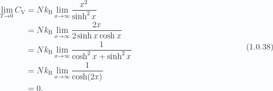
Low temperature limits

For the classical case the heat capacity was constant (C_{\mathrm{V}} = N k_{\mathrm{B}}), all the way down to zero. For the quantum case the heat capacity drops to zero for low temperatures. We can see that via L’hopitals rule. With x = \hbar \omega \beta/2 the low temperature limit is

\begin{aligned}\lim_{T \rightarrow 0} C_{\mathrm{V}} &= N k_{\mathrm{B}} \lim_{x \rightarrow \infty} \frac{x^2}{\sinh^2 x} \\ &= N k_{\mathrm{B}} \lim_{x \rightarrow \infty} \frac{2x }{2 \sinh x \cosh x} \\ &= N k_{\mathrm{B}} \lim_{x \rightarrow \infty} \frac{1 }{\cosh^2 x + \sinh^2 x} \\ &= N k_{\mathrm{B}} \lim_{x \rightarrow \infty} \frac{1 }{\cosh (2 x) } \\ &= 0.\end{aligned} \hspace{\stretch{1}}(1.0.38)

We also see this in the plot of fig. 1.2.

Fig 1.2: Specific heat for N quantum oscillators

Question: Quantum electric dipole (2013 problem set 5, p3)

A quantum electric dipole at a fixed space point has its energy determined by two parts – a part which comes from its angular motion and a part coming from its interaction with an applied electric field \mathcal{E}. This leads to a quantum Hamiltonian

\begin{aligned}H = \frac{\mathbf{L} \cdot \mathbf{L}}{2 I} - \mu \mathcal{E} L_z,\end{aligned} \hspace{\stretch{1}}(1.0.39)

where I is the moment of inertia, and we have assumed an electric field \mathcal{E} = \mathcal{E} \hat{\mathbf{z}}. This Hamiltonian has eigenstates described by spherical harmonics Y_{l, m}(\theta, \phi), with m taking on 2l+1 possible integral values, m = -l, -l + 1, \cdots, l -1, l. The corresponding eigenvalues are

\begin{aligned}\lambda_{l, m} = \frac{l(l+1) \hbar^2}{2I} - \mu \mathcal{E} m \hbar.\end{aligned} \hspace{\stretch{1}}(1.0.40)

(Recall that l is the total angular momentum eigenvalue, while m is the eigenvalue corresponding to L_z.)

Part a

Schematically sketch these eigenvalues as a function of \mathcal{E} for l = 0,1,2.

Part b

Find the quantum partition function, assuming only l = 0 and l = 1 contribute to the sum.

Part c

Using this partition function, find the average dipole moment \mu \left\langle{{L_z}}\right\rangle as a function of the electric field and temperature for small electric fields, commenting on its behavior at very high temperature and very low temperature.

Part d

Estimate the temperature above which discarding higher angular momentum states, with l \ge 2, is not a good approximation.

Answer

Sketch the energy eigenvalues

Let’s summarize the values of the energy eigenvalues \lambda_{l,m} for l = 0, 1, 2 before attempting to plot them.

l = 0

For l = 0, the azimuthal quantum number can only take the value m = 0, so we have

\begin{aligned}\lambda_{0,0} = 0.\end{aligned} \hspace{\stretch{1}}(1.0.41)

l = 1

For l = 1 we have

\begin{aligned}\frac{l(l+1)}{2} = 1(2)/2 = 1,\end{aligned} \hspace{\stretch{1}}(1.0.42)

so we have

\begin{aligned}\lambda_{1,0} = \frac{\hbar^2}{I} \end{aligned} \hspace{\stretch{1}}(1.0.43a)

\begin{aligned}\lambda_{1,\pm 1} = \frac{\hbar^2}{I} \mp \mu \mathcal{E} \hbar.\end{aligned} \hspace{\stretch{1}}(1.0.43b)

l = 2

For l = 2 we have

\begin{aligned}\frac{l(l+1)}{2} = 2(3)/2 = 3,\end{aligned} \hspace{\stretch{1}}(1.0.44)

so we have

\begin{aligned}\lambda_{2,0} = \frac{3 \hbar^2}{I} \end{aligned} \hspace{\stretch{1}}(1.0.45a)

\begin{aligned}\lambda_{2,\pm 1} = \frac{3 \hbar^2}{I} \mp \mu \mathcal{E} \hbar\end{aligned} \hspace{\stretch{1}}(1.0.45b)

\begin{aligned}\lambda_{2,\pm 2} = \frac{3 \hbar^2}{I} \mp 2 \mu \mathcal{E} \hbar.\end{aligned} \hspace{\stretch{1}}(1.0.45c)

These are sketched as a function of \mathcal{E} in fig. 1.3.

Fig 1.3: Energy eigenvalues for l = 0,1, 2

Partition function

Our partition function, in general, is
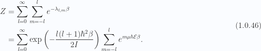
\begin{aligned}Z &= \sum_{l = 0}^\infty \sum_{m = -l}^l e^{-\lambda_{l,m} \beta} \\ &= \sum_{l = 0}^\infty \exp\left( -\frac{l (l+1) \hbar^2 \beta}{2 I} \right)\sum_{m = -l}^l e^{ m \mu \hbar \mathcal{E} \beta}.\end{aligned} \hspace{\stretch{1}}(1.0.46)

Dropping all but l = 0, 1 terms this is

\begin{aligned}Z \approx 1 + e^{-\hbar^2 \beta/I} \left( 1 + e^{- \mu \hbar \mathcal{E} \beta } + e^{ \mu \hbar \mathcal{E} \beta} \right),\end{aligned} \hspace{\stretch{1}}(1.0.47)

or

\begin{aligned}\boxed{Z \approx 1 + e^{-\hbar^2 \beta/I} (1 + 2 \cosh\left( \mu \hbar \mathcal{E} \beta \right)).}\end{aligned} \hspace{\stretch{1}}(1.0.48)

Average dipole moment

For the average dipole moment, averaging over both the states and the partitions, we have
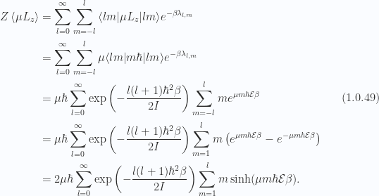
\begin{aligned}Z \left\langle{{ \mu L_z }}\right\rangle &= \sum_{l = 0}^\infty \sum_{m = -l}^l {\left\langle {l m} \right\rvert} \mu L_z {\left\lvert {l m} \right\rangle} e^{-\beta \lambda_{l, m}} \\ &= \sum_{l = 0}^\infty \sum_{m = -l}^l \mu {\left\langle {l m} \right\rvert} m \hbar {\left\lvert {l m} \right\rangle} e^{-\beta \lambda_{l, m}} \\ &= \mu \hbar \sum_{l = 0}^\infty \exp\left( -\frac{l (l+1) \hbar^2 \beta}{2 I} \right)\sum_{m = -l}^l m e^{ \mu m \hbar \mathcal{E} \beta} \\ &= \mu \hbar \sum_{l = 0}^\infty \exp\left( -\frac{l (l+1) \hbar^2 \beta}{2 I} \right)\sum_{m = 1}^l m \left( e^{ \mu m \hbar \mathcal{E} \beta} -e^{-\mu m \hbar \mathcal{E} \beta} \right) \\ &= 2 \mu \hbar \sum_{l = 0}^\infty \exp\left( -\frac{l (l+1) \hbar^2 \beta}{2 I} \right)\sum_{m = 1}^l m \sinh (\mu m \hbar \mathcal{E} \beta).\end{aligned} \hspace{\stretch{1}}(1.0.49)

For the cap of l = 1 we have

\begin{aligned}\left\langle{{ \mu L_z }}\right\rangle \approx\frac{2 \mu \hbar }{Z}\left( 1 (0) + e^{-\hbar^2 \beta/ I} \sinh (\mu \hbar \mathcal{E} \beta) \right)\approx2 \mu \hbar \frac{e^{-\hbar^2 \beta/ I} \sinh (\mu \hbar \mathcal{E} \beta) }{1 + e^{-\hbar^2 \beta/I} \left( 1 + 2 \cosh( \mu \hbar \mathcal{E} \beta) \right)},\end{aligned} \hspace{\stretch{1}}(1.0.50)

or

\begin{aligned}\boxed{\left\langle{{ \mu L_z }}\right\rangle \approx\frac{2 \mu \hbar \sinh (\mu \hbar \mathcal{E} \beta) }{e^{\hbar^2 \beta/I} + 1 + 2 \cosh( \mu \hbar \mathcal{E} \beta)}.}\end{aligned} \hspace{\stretch{1}}(1.0.51)

This is plotted in fig. 1.4.

Fig 1.4: Dipole moment

For high temperatures \mu \hbar \mathcal{E} \beta \ll 1 or k_{\mathrm{B}} T \gg \mu \hbar \mathcal{E}, expanding the hyperbolic sine and cosines to first and second order respectively and the exponential to first order we have

\begin{aligned}\left\langle{{ \mu L_z }}\right\rangle &\approx 2 \mu \hbar \frac{ \frac{\mu \hbar \mathcal{E}}{k_{\mathrm{B}} T}}{ 4 + \frac{h^2}{I k_{\mathrm{B}} T} + \left( \frac{\mu \hbar \mathcal{E}}{k_{\mathrm{B}} T} \right)^2}=\frac{2 (\mu \hbar)^2 \mathcal{E} k_{\mathrm{B}} T}{4 (k_{\mathrm{B}} T)^2 + \hbar^2 k_{\mathrm{B}} T/I + (\mu \hbar \mathcal{E})^2 } \\ &\approx\frac{(\mu \hbar)^2 \mathcal{E}}{4 k_{\mathrm{B}} T}.\end{aligned} \hspace{\stretch{1}}(1.0.52)

Our dipole moment tends to zero approximately inversely proportional to temperature. These last two respective approximations are plotted along with the all temperature range result in fig. 1.5.

Fig 1.5: High temperature approximations to dipole moments

For low temperatures k_{\mathrm{B}} T \ll \mu \hbar \mathcal{E}, where \mu \hbar \mathcal{E} \beta \gg 1 we have

\begin{aligned}\left\langle{{ \mu L_z }}\right\rangle \approx\frac{ 2 \mu \hbar e^{\mu \hbar \mathcal{E} \beta} }{ e^{\hbar^2 \beta/I} + e^{\mu \hbar \mathcal{E} \beta} }=\frac{ 2 \mu \hbar }{ 1 + e^{ (\hbar^2 \beta/I - \mu \hbar \mathcal{E})/{k_{\mathrm{B}} T} } }.\end{aligned} \hspace{\stretch{1}}(1.0.53)

Provided the electric field is small enough (which means here that \mathcal{E} < \hbar/\mu I) this will look something like fig. 1.6.

Fig 1.6: Low temperature dipole moment behavior

Approximation validation

In order to validate the approximation, let’s first put the partition function and the numerator of the dipole moment into a tidier closed form, evaluating the sums over the radial indices l. First let’s sum the exponentials for the partition function, making an n = m + l

\begin{aligned}\sum_{m = -l}^l a^m &= a^{-l} \sum_{n=0}^{2l} a^n \\ &= a^{-l} \frac{a^{2l + 1} - 1}{a - 1} \\ &= \frac{a^{l + 1} - a^{-l}}{a - 1} \\ &= \frac{a^{l + 1/2} - a^{-(l+1/2)}}{a^{1/2} - a^{-1/2}}.\end{aligned} \hspace{\stretch{1}}(1.0.54)

With a substitution of a = e^b, we have

\begin{aligned}\boxed{\sum_{m = -l}^l e^{b m}=\frac{\sinh(b(l + 1/2))}{\sinh(b/2)}.}\end{aligned} \hspace{\stretch{1}}(1.0.55)

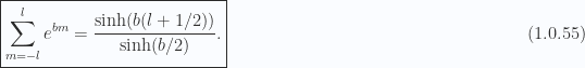
Now we can sum the azimuthal exponentials for the dipole moment. This sum is of the form

\begin{aligned}\sum_{m = -l}^l m a^m &= a \left( \sum_{m = 1}^l + \sum_{m = -l}^{-1} \right)m a^{m-1} \\ &= a \frac{d}{da}\sum_{m = 1}^l\left( a^{m} + a^{-m} \right) \\ &= a \frac{d}{da}\left( \sum_{m = -l}^l a^m - \not{{1}} \right) \\ &= a \frac{d}{da}\left( \frac{a^{l + 1/2} - a^{-(l+1/2)}}{a^{1/2} - a^{-1/2}} \right).\end{aligned} \hspace{\stretch{1}}(1.0.56)

With a = e^{b}, and 1 = a db/da, we have

\begin{aligned}a \frac{d}{da} = a \frac{db}{da} \frac{d}{db} = \frac{d}{db},\end{aligned} \hspace{\stretch{1}}(1.0.57)

we have

\begin{aligned}\sum_{m = -l}^l m e^{b m}= \frac{d}{db}\left( \frac{ \sinh(b(l + 1/2)) }{ \sinh(b/2) } \right).\end{aligned} \hspace{\stretch{1}}(1.0.58)

With a little help from Mathematica to simplify that result we have

\begin{aligned}\boxed{\sum_{m = -l}^l m e^{b m}=\frac{l \sinh(b (l+1)) - (l+1) \sinh(b l) }{2 \sinh^2(b/2)}.}\end{aligned} \hspace{\stretch{1}}(1.0.59)

We can now express the average dipole moment with only sums over radial indices l

\begin{aligned}\left\langle{{ \mu L_z }}\right\rangle &= \mu \hbar \frac{ \sum_{l = 0}^\infty \exp\left( -\frac{l (l+1) \hbar^2 \beta}{2 I} \right) \sum_{m = -l}^l m e^{ \mu m \hbar \mathcal{E} \beta}}{ \sum_{l = 0}^\infty \exp\left( -\frac{l (l+1) \hbar^2 \beta}{2 I} \right) \sum_{m = -l}^l e^{ m \mu \hbar \mathcal{E} \beta}} \\ &= \mu \hbar\frac{ \sum_{l = 0}^\infty \exp\left( -\frac{l (l+1) \hbar^2 \beta}{2 I} \right) \frac { l \sinh(\mu \hbar \mathcal{E} \beta (l+1)) - (l+1) \sinh(\mu \hbar \mathcal{E} \beta l) } { 2 \sinh^2(\mu \hbar \mathcal{E} \beta/2) }}{\sum_{l = 0}^\infty \exp\left( -\frac{l (l+1) \hbar^2 \beta}{2 I} \right) \frac { \sinh(\mu \hbar \mathcal{E} \beta(l + 1/2)) } { \sinh(\mu \hbar \mathcal{E} \beta/2) }}.\end{aligned} \hspace{\stretch{1}}(1.0.60)

So our average dipole moment is

\begin{aligned}\boxed{\left\langle{{ \mu L_z }}\right\rangle = \frac{\mu \hbar }{2 \sinh(\mu \hbar \mathcal{E} \beta/2)}\frac{ \sum_{l = 0}^\infty \exp\left( -\frac{l (l+1) \hbar^2 \beta}{2 I} \right)\left( l \sinh(\mu \hbar \mathcal{E} \beta (l+1)) - (l+1) \sinh(\mu \hbar \mathcal{E} \beta l) \right)}{ \sum_{l = 0}^\infty \exp\left( -\frac{l (l+1) \hbar^2 \beta}{2 I} \right) \sinh(\mu \hbar \mathcal{E} \beta(l + 1/2))}.}\end{aligned} \hspace{\stretch{1}}(1.0.61)

The hyperbolic sine in the denominator from the partition function and the difference of hyperbolic sines in the numerator both grow fast. This is illustrated in fig. 1.7.

Fig 1.7: Hyperbolic sine plots for dipole moment

Let’s look at the order of these hyperbolic sines for large arguments. For the numerator we have a difference of the form

\begin{aligned}x \sinh( x + 1 ) - (x + 1) \sinh ( x ) &= \frac{1}{{2}} \left( x \left( e^{x + 1} - e^{-x - 1} \right) -(x +1 ) \left( e^{x } - e^{-x } \right) \right)\approx\frac{1}{{2}} \left( x e^{x + 1} -(x +1 ) e^{x } \right) \\ &= \frac{1}{{2}} \left( x e^{x} ( e - 1 ) - e^x \right) \\ &= O(x e^x).\end{aligned} \hspace{\stretch{1}}(1.0.62)

For the hyperbolic sine from the partition function we have for large x

\begin{aligned}\sinh( x + 1/2) = \frac{1}{{2}} \left( e^{x + 1/2} - e^{-x - 1/2} \right)\approx \frac{\sqrt{e}}{2} e^{x}= O(e^x).\end{aligned} \hspace{\stretch{1}}(1.0.63)

While these hyperbolic sines increase without bound as l increases, we have a negative quadratic dependence on l in the \mathbf{L}^2 contribution to these sums, provided that is small enough we can neglect the linear growth of the hyperbolic sines. We wish for that factor to be large enough that it dominates for all l. That is

\begin{aligned}\frac{l(l+1) \hbar^2}{2 I k_{\mathrm{B}} T} \gg 1,\end{aligned} \hspace{\stretch{1}}(1.0.64)

or

\begin{aligned}T \ll \frac{l(l+1) \hbar^2}{2 I k_{\mathrm{B}} T}.\end{aligned} \hspace{\stretch{1}}(1.0.65)

Observe that the RHS of this inequality, for l = 1, 2, 3, 4, \cdots satisfies

\begin{aligned}\frac{\hbar^2 }{I k_{\mathrm{B}}}<\frac{3 \hbar^2 }{I k_{\mathrm{B}}}<\frac{6 \hbar^2 }{I k_{\mathrm{B}}}<\frac{10 \hbar^2 }{I k_{\mathrm{B}}}< \cdots\end{aligned} \hspace{\stretch{1}}(1.0.66)

So, for small electric fields, our approximation should be valid provided our temperature is constrained by

\begin{aligned}\boxed{T \ll \frac{\hbar^2 }{I k_{\mathrm{B}}}.}\end{aligned} \hspace{\stretch{1}}(1.0.67)

Posted in Math and Physics Learning. | Tagged: , , , , , , , , , , , , , , , , , , , , , , , , | Leave a Comment »

PHY452H1S Basic Statistical Mechanics. Problem Set 4: Ideal gas

Posted by peeterjoot on March 3, 2013

[Click here for a PDF of this post with nicer formatting]

Disclaimer

This is an ungraded set of answers to the problems posed.

Question: Sackur-Tetrode entropy of an Ideal Gas

The entropy of an ideal gas is given by

\begin{aligned}S = N k_{\mathrm{B}}\left( \ln \left( \frac{V}{N} \left( \frac{4 \pi m E}{3 N h^2} \right) ^{3/2} \right) + \frac{5}{2} \right)\end{aligned} \hspace{\stretch{1}}(1.1.1)

Find the temperature of this gas via (\partial S/ \partial E)_{V,N} = 1/T. Find the energy per particle at which the entropy becomes negative. Is there any meaning to this temperature?

Answer

Taking derivatives we find

\begin{aligned}\frac{1}{{T}} &= \frac{\partial {}}{\partial {E}}\left( \not{{ N k_{\mathrm{B}} \ln \frac{V}{N} }} + N k_{\mathrm{B}} \frac{3}{2} \ln \left( \frac{4 \pi m E}{3 N h^2} \right) + \not{{N k_{\mathrm{B}} \frac{5}{2} }} \right) \\ &= \frac{3}{2} N k_{\mathrm{B}} \frac{1}{{E}}\end{aligned} \hspace{\stretch{1}}(1.1.2)

or

\begin{aligned}\boxed{T = \frac{2}{3} \frac{E}{N k_{\mathrm{B}} }}\end{aligned} \hspace{\stretch{1}}(1.1.3)

The energies for which the entropy is negative are given by

\begin{aligned}\left( \frac{4 \pi m E}{3 N h^2} \right)^{3/2}\le \frac{N}{V} e^{-5/2},\end{aligned} \hspace{\stretch{1}}(1.1.4)

or

\begin{aligned}E &\le \frac{3 N h^2}{4 \pi m} \left( \frac{N}{V e^{5/2}} \right)^{2/3} \\ &= \frac{3 h^2 N^{5/3}}{4 \pi m V^{2/3} e^{5/2}}.\end{aligned} \hspace{\stretch{1}}(1.1.5)

In terms of the temperature T this negative entropy condition is given by

\begin{aligned}\not{{\frac{3 N}{2}}} k_{\mathrm{B}} T \le \not{{\frac{3 N}{2}}} \left( \frac{ N}{V} \right)^{2/3} \frac{h^2}{e^{5/2}},\end{aligned} \hspace{\stretch{1}}(1.1.6)

or

\begin{aligned}\boxed{\frac{\sqrt{2 \pi m k_{\mathrm{B}} T}}{h} \le \left( \frac{N}{V} \right)^{1/3} \frac{1}{{e^{5/4}}}.}\end{aligned} \hspace{\stretch{1}}(1.1.7)

There will be a particle density V/N for which this distance h/\sqrt{2 \pi m k_{\mathrm{B}} T} will start approaching the distance between atoms. This distance constrains the validity of the ideal gas law entropy equation. Putting this quantity back into the entropy eq. 1.1.1 we have

\begin{aligned}\frac{S}{N k_{\mathrm{B}}} = \ln \frac{V}{N} \left( \frac{\sqrt{2 \pi m k_{\mathrm{B}} T}}{h} \right)^3 + \frac{5}{2}\end{aligned} \hspace{\stretch{1}}(1.1.8)

We see that a positive entropy requirement puts a bound on this distance (as a function of temperature) since we must also have

\begin{aligned}\frac{h}{\sqrt{2 \pi m k_{\mathrm{B}} T}} \ll \left( \frac{V}{N} \right)^{1/3},\end{aligned} \hspace{\stretch{1}}(1.1.9)

for the gas to be in the classical domain. I’d actually expect a gas to liquefy before this transition point, making such a low temperature nonphysical. To get a feel for whether this is likely the case, we should expect that the logarithm argument to be

\begin{aligned}\frac{V}{N} \left( \frac{\sqrt{2 \pi m k_{\mathrm{B}} T}}{h} \right)^3\end{aligned} \hspace{\stretch{1}}(1.1.10)

at the point where gasses liquefy (at which point we assume the ideal gas law is no longer accurate) to be well above unity. Checking this for 1 liter of a gas with 10^23 atoms for hydrogen, helium, and neon respectively we find the values for eq. 1.1.10 are

\begin{aligned}173.682, 130.462, 23993.\end{aligned} \hspace{\stretch{1}}(1.1.11)

At least for these first few cases we see that the ideal gas law has lost its meaning well before the temperatures below which the entropy would become negative.

Question: Ideal gas thermodynamics

An ideal gas starts at (V_0, P_0) in the pressure-volume diagram (x-axis = V, y-axis = P), then moves at constant pressure to a larger volume (V_1, P_0), then moves to a larger pressure at constant volume to (V_1, P_1), and finally returns to (V_0, P_0), thus undergoing a cyclic process (forming a triangle in P-V plane). For each step, find the work done on the gas, the change in energy content, and heat added to the gas. Find the total work/energy/heat change over the entire cycle.

Answer

Our process is illustrated in fig. 1.1.

Fig 1.1: Cyclic pressure volume process

Step 1
This problem is somewhat underspecified. From the ideal gas law, regardless of how the gas got from the initial to the final states, we have

\begin{aligned}P_0 V_0 = N_0 k_{\mathrm{B}} T_0\end{aligned} \hspace{\stretch{1}}(1.0.12a)

\begin{aligned}P_0 V_1 = N_1 k_{\mathrm{B}} T_1\end{aligned} \hspace{\stretch{1}}(1.0.12b)

So a volume increase with fixed P implies that there is a corresponding increase in N T. We could have for example, an increase in the number of particles, as in the evaporation process illustrated of fig. 1.2, where a piston held down by (fixed) atmospheric pressure is pushed up as the additional gas boils off.

Fig 1.2: Evaporation process under (fixed) atmospheric pressure

Alternately, we could have a system such as that of fig. 1.3, with a fixed amount of gas is in contact with a heat source that supplies the energy required to induce the required increase in temperature.

Fig 1.3: Gas of fixed mass absorbing heat

Regardless of the source of the energy that accounts for the increase in volume the work done on the gas (a negation of the positive work the gas is performing on the system, perhaps a piston as in the picture) is

\begin{aligned}d W_1 = - \int_{V_0}^{V_1} p dV = -P_0 (V_1 - V_0).\end{aligned} \hspace{\stretch{1}}(1.0.13)

Let’s now assume that we have the second sort of configuration above, where the total amount of gas is held fixed. From the ideal gas relations of eq. 1.0.12.12, and with \Delta V = V_1 - V_0, \Delta T = T_1 - T_0, and N_1 = N_0 = N, we have

\begin{aligned}P_0 \Delta V = N k_{\mathrm{B}} \Delta T.\end{aligned} \hspace{\stretch{1}}(1.0.14)

The change in energy of the ideal gas, assuming three degrees of freedom, is

\begin{aligned}d U = \frac{3}{2} N k_{\mathrm{B}} \Delta T = \frac{3}{2} P_0 \Delta V.\end{aligned} \hspace{\stretch{1}}(1.0.15)

The energy balance then requires that the total heat absorbed by the gas must include that portion that has done work on the system, plus the excess kinetic energy of the gas. That is

\begin{aligned}d Q_1 &= \frac{3}{2} P_0 \Delta V + P_0 \Delta V \\ &= \frac{5}{2} P_0 \Delta V.\end{aligned} \hspace{\stretch{1}}(1.0.16)

Step 2

For this leg of the cycle we have no work done on the gas

\begin{aligned}d W_2 = -\int_{V_1}^{V_1} P dV = 0.\end{aligned} \hspace{\stretch{1}}(1.0.17)

We do, however have a change in energy. The energy of the gas is

\begin{aligned}U = \frac{3}{2} N k_b T = \frac{3}{2} P V.\end{aligned} \hspace{\stretch{1}}(1.0.18)

With \Delta P = P_1 - P_0, the change of energy of the gas, the total heat absorbed by the gas, is

\begin{aligned}dU_2 = d Q_2 = \frac{3}{2} V_1 \Delta P.\end{aligned} \hspace{\stretch{1}}(1.0.19)

Step 3

For the final leg of the cycle, the work done on the gas is

\begin{aligned}d W_3 &= -\int_{V_1}^{V_0} P dV \\ &= \int_{V_0}^{V_1} P dV \\ &= \Delta V \frac{P_0 + P_1}{2}.\end{aligned} \hspace{\stretch{1}}(1.0.20)

This is positive this time
Unlike the first part of the cycle, the work done on the gas is positive this time (work is being done on the gas to both compress it). The change in energy of the gas, however, is negative, with the difference between final and initial energy being

\begin{aligned}dU_3 &= \frac{3}{2} (P_0 V_0 - P_1 V_1)  \\ &= -\frac{3}{2} (P_1 V_1 - P_0 V_0) <0.\end{aligned} \hspace{\stretch{1}}(1.0.21)

The simultaneous compression and the pressure reduction require energy to be removed from the gas. We must have a negative change in heat d Q < 0, with heat emitted in this phase of the cycle. This can be verified explicitly

\begin{aligned}d Q_3 &= dU - d W \\ &= -\frac{3}{2} (P_1 V_1 - P_0 V_0) - \frac{1}{{2}} \Delta V (P_1 + P_0)< 0.\end{aligned} \hspace{\stretch{1}}(1.0.22)

Changes over the complete cycle.

Summarizing the results from each of the phases, we have

\begin{aligned}d W_1 = -P_0 \Delta V\end{aligned} \hspace{\stretch{1}}(1.0.23a)

\begin{aligned}d Q_1 = \frac{5}{2} P_0 \Delta V \end{aligned} \hspace{\stretch{1}}(1.0.23b)

\begin{aligned}d U_1 = \frac{3}{2} P_0 \Delta V \end{aligned} \hspace{\stretch{1}}(1.0.23c)

\begin{aligned}d W_2 = 0 \end{aligned} \hspace{\stretch{1}}(1.0.24a)

\begin{aligned}d Q_2 = \frac{3}{2} V_1 \Delta P \end{aligned} \hspace{\stretch{1}}(1.0.24b)

\begin{aligned}d U_2 = \frac{3}{2} V_1 \Delta P \end{aligned} \hspace{\stretch{1}}(1.0.24c)

\begin{aligned}d W_3 = \Delta V \frac{P_0 + P_1}{2} \end{aligned} \hspace{\stretch{1}}(1.0.25a)

\begin{aligned}d Q_3 = -\frac{1}{{2}} ( 3(P_1 V_1 - P_0 V_0) + \Delta V (P_1 + P_0)) \end{aligned} \hspace{\stretch{1}}(1.0.25b)

\begin{aligned}d U_3 = -\frac{3}{2} ( P_1 V_1 - P_0 V_0 )\end{aligned} \hspace{\stretch{1}}(1.0.25c)

Summing the changes in the work we have

\begin{aligned}\sum_{i = 1}^3 d W_i = \frac{1}{{2}} \Delta V \Delta P > 0.\end{aligned} \hspace{\stretch{1}}(1.0.26)

This is the area of the triangle, as expected. Since it is positive, there is net work done on the gas.

We expect the energy changes to sum to zero, and this can be verified explicitly finding

\begin{aligned}\sum_{i = 1}^3 d U_i &= \frac{3}{2} P_0 \Delta V -\frac{3}{2} ( P_1 V_1 - P_0 V_0 ) \\ &= 0.\end{aligned} \hspace{\stretch{1}}(1.0.27)

With net work done on the gas and no change in energy, there should be no net heat absorption by the gas, with a total change in heat that should equal, in amplitude, the total work done on the gas. This is confirmed by summation

\begin{aligned}\sum_{i = 1}^3 d Q_i &= \frac{5}{2} P_0 \Delta V +\frac{3}{2} V_1 \Delta P -\frac{1}{{2}} ( 3(P_1 V_1 - P_0 V_0) + \Delta V (P_1 + P_0)) \\ &= -\frac{1}{{2}} \Delta P \Delta V.\end{aligned} \hspace{\stretch{1}}(1.0.28)

Question: Adiabatic process for an Ideal Gas

Show that when an ideal monoatomic gas expands adiabatically, the temperature and pressure are related by

\begin{aligned}\frac{dT}{dP}=\frac{2}{5}\frac{T}{P}\end{aligned} \hspace{\stretch{1}}(1.0.29)

Answer

From (3.34b) of [1], we find that the Adiabatic condition can be expressed algebraically as

\begin{aligned}0 = d Q = T dS = dU + P dV.\end{aligned} \hspace{\stretch{1}}(1.0.30)

With

\begin{aligned}U = \frac{3}{2} N k_{\mathrm{B}} T = \frac{3}{2} P V,\end{aligned} \hspace{\stretch{1}}(1.0.31)

this is

\begin{aligned}0 &= \frac{3}{2} V dP + \frac{3}{2} P dV + P dV \\ &= \frac{3}{2} V dP + \frac{5}{2} P dV.\end{aligned} \hspace{\stretch{1}}(1.0.32)

Dividing through by P V, this becomes a perfect differential, and we can integrate

\begin{aligned}0 &= 3 \int \frac{dP }{P}+ 5 \int \frac{dV}{V} \\ &= 3 \ln P + 5 \ln V + \ln C \\ &= 3 \ln PV + 2 \ln V + \ln C \\ &= \ln (N k_{\mathrm{B}} T)^3 + \ln \left( \frac{N k_{\mathrm{B}} T}{P} \right)^2 + \ln C.\end{aligned} \hspace{\stretch{1}}(1.0.33)

Exponentiating yields

\begin{aligned}T^5 = C' P^2.\end{aligned} \hspace{\stretch{1}}(1.0.34)

The desired relation follows by taking derivatives

\begin{aligned}2 C' P &= 5 T^4 \frac{dT}{dP} \\ &= 5 C' \frac{P^2}{T} \frac{dT}{dP},\end{aligned} \hspace{\stretch{1}}(1.0.35)

or

\begin{aligned}\frac{dT}{dP} =\frac{2}{5} \frac{T}{P},\end{aligned} \hspace{\stretch{1}}(1.0.36)

as desired.

References

[1] C. Kittel and H. Kroemer. Thermal physics. WH Freeman, 1980.

Posted in Math and Physics Learning. | Tagged: , , , , , , , , , | Leave a Comment »