[Click here for a PDF of this post with nicer formatting]
Disclaimer.
This problem set is as yet ungraded (although only the second question will be graded).
Problem 1. Fun with  ,
,  ,
,  , and the duality of Maxwell’s equations in vacuum.
1. Statement. rank 3 spatial antisymmetric tensor identities.
Prove that

and use it to find the familiar relation for

Also show that

(Einstein summation implied all throughout this problem).
1. Solution
We can explicitly expand the (implied) sum over indexes  . This is

For any  only one term is non-zero. For example with
  , we have just a contribution from the
  part of the sum

The value of this for  is
is

whereas for  we have

Our sum has value one when  matches
  , and value minus one for when are permuted. We can summarize this, by saying that when we have

However, observe that when  the RHS is

as desired, so this form works in general without any qualifier, completing this part of the problem.

This gives us

We have one more identity to deal with.

We can expand out this (implied) sum slow and dumb as well

Now, observe that for any  only one term of this sum is picked up. For example, with no loss of generality, pick
  . We are left with only

This has the value

when  and is zero otherwise. We can therefore summarize the evaluation of this sum as

completing this problem.
2. Statement. Determinant of three by three matrix.
Prove that for any  matrix
  :
:  and that
  .
.
2. Solution
In class Simon showed us how the first identity can be arrived at using the triple product  . It occurred to me later that I’d seen the identity to be proven in the context of Geometric Algebra, but hadn’t recognized it in this tensor form. Basically, a wedge product can be expanded in sums of determinants, and when the dimension of the space is the same as the vector, we have a pseudoscalar times the determinant of the components.
For example, in  , let’s take the wedge product of a pair of vectors. As preparation for the relativistic
  case We won’t require an orthonormal basis, but express the vector in terms of a reciprocal frame and the associated components

where

When we get to the relativistic case, we can pick (but don’t have to) the standard basis

for which our reciprocal frame is implicitly defined by the metric

Anyways. Back to the problem. Let’s examine the case. Our wedge product in coordinates is

Since there are only two basis vectors we have

Our wedge product is a product of the determinant of the vector coordinates, times the pseudoscalar  .
.
This doesn’t look quite like the  relation that we want to prove, which had an antisymmetric tensor factor for the determinant. Observe that we get the determinant by picking off the component of the bivector result (the only component in this case), and we can do that by dotting with
  . To get an antisymmetric tensor times the determinant, we have only to dot with a different pseudoscalar (one that differs by a possible sign due to permutation of the indexes). That is
![\begin{aligned}(e^t \wedge e^s) \cdot (a \wedge b)&=a^i b^j (e^t \wedge e^s) \cdot (e_i \wedge e_j) \\ &=a^i b^j\left( {\delta^{s}}_i {\delta^{t}}_j-{\delta^{t}}_i {\delta^{s}}_j \right) \\ &=a^i b^j{\delta^{[t}}_j {\delta^{s]}}_i \\ &=a^i b^j{\delta^{t}}_{[j} {\delta^{s}}_{i]} \\ &=a^{[i} b^{j]}{\delta^{t}}_{j} {\delta^{s}}_{i} \\ &=a^{[s} b^{t]}\end{aligned}](https://s0.wp.com/latex.php?latex=%5Cbegin%7Baligned%7D%28e%5Et+%5Cwedge+e%5Es%29+%5Ccdot+%28a+%5Cwedge+b%29%26%3Da%5Ei+b%5Ej+%28e%5Et+%5Cwedge+e%5Es%29+%5Ccdot+%28e_i+%5Cwedge+e_j%29+%5C%5C+%26%3Da%5Ei+b%5Ej%5Cleft%28+%7B%5Cdelta%5E%7Bs%7D%7D_i+%7B%5Cdelta%5E%7Bt%7D%7D_j-%7B%5Cdelta%5E%7Bt%7D%7D_i+%7B%5Cdelta%5E%7Bs%7D%7D_j++%5Cright%29+%5C%5C+%26%3Da%5Ei+b%5Ej%7B%5Cdelta%5E%7B%5Bt%7D%7D_j+%7B%5Cdelta%5E%7Bs%5D%7D%7D_i+%5C%5C+%26%3Da%5Ei+b%5Ej%7B%5Cdelta%5E%7Bt%7D%7D_%7B%5Bj%7D+%7B%5Cdelta%5E%7Bs%7D%7D_%7Bi%5D%7D+%5C%5C+%26%3Da%5E%7B%5Bi%7D+b%5E%7Bj%5D%7D%7B%5Cdelta%5E%7Bt%7D%7D_%7Bj%7D+%7B%5Cdelta%5E%7Bs%7D%7D_%7Bi%7D+%5C%5C+%26%3Da%5E%7B%5Bs%7D+b%5E%7Bt%5D%7D%5Cend%7Baligned%7D+&bg=fafcff&fg=2a2a2a&s=0&c=20201002)
Now, if we write  and
and  we have

We can write this in two different ways. One of which is

and the other of which is by introducing free indexes for  and
and  , and summing antisymmetrically over these. That is

So, we have
![\begin{aligned}\boxed{A^{a s} A^{b t} \epsilon_{a b} =A^{1 i} A^{2 j} {\delta^{[t}}_j {\delta^{s]}}_i =\epsilon^{s t} \text{Det} {\left\lVert{A^{ij}}\right\rVert},}\end{aligned} \hspace{\stretch{1}}(2.30)](https://s0.wp.com/latex.php?latex=%5Cbegin%7Baligned%7D%5Cboxed%7BA%5E%7Ba+s%7D+A%5E%7Bb+t%7D+%5Cepsilon_%7Ba+b%7D+%3DA%5E%7B1+i%7D+A%5E%7B2+j%7D+%7B%5Cdelta%5E%7B%5Bt%7D%7D_j+%7B%5Cdelta%5E%7Bs%5D%7D%7D_i+%3D%5Cepsilon%5E%7Bs+t%7D+%5Ctext%7BDet%7D+%7B%5Cleft%5ClVert%7BA%5E%7Bij%7D%7D%5Cright%5CrVert%7D%2C%7D%5Cend%7Baligned%7D+%5Chspace%7B%5Cstretch%7B1%7D%7D%282.30%29&bg=fafcff&fg=2a2a2a&s=0&c=20201002)
This result hold regardless of the metric for the space, and does not require that we were using an orthonormal basis. When the metric is Euclidean and we have an orthonormal basis, then all the indexes can be dropped.
The and cases follow in exactly the same way, we just need more vectors in the wedge products.
For the case we have
![\begin{aligned}(e^u \wedge e^t \wedge e^s) \cdot ( a \wedge b \wedge c)&=a^i b^j c^k(e^u \wedge e^t \wedge e^s) \cdot (e_i \wedge e_j \wedge e_k) \\ &=a^i b^j c^k{\delta^{[u}}_k{\delta^{t}}_j{\delta^{s]}}_i \\ &=a^{[s} b^t c^{u]}\end{aligned}](https://s0.wp.com/latex.php?latex=%5Cbegin%7Baligned%7D%28e%5Eu+%5Cwedge+e%5Et+%5Cwedge+e%5Es%29+%5Ccdot+%28+a+%5Cwedge+b+%5Cwedge+c%29%26%3Da%5Ei+b%5Ej+c%5Ek%28e%5Eu+%5Cwedge+e%5Et+%5Cwedge+e%5Es%29+%5Ccdot+%28e_i+%5Cwedge+e_j+%5Cwedge+e_k%29+%5C%5C+%26%3Da%5Ei+b%5Ej+c%5Ek%7B%5Cdelta%5E%7B%5Bu%7D%7D_k%7B%5Cdelta%5E%7Bt%7D%7D_j%7B%5Cdelta%5E%7Bs%5D%7D%7D_i+%5C%5C+%26%3Da%5E%7B%5Bs%7D+b%5Et+c%5E%7Bu%5D%7D%5Cend%7Baligned%7D+&bg=fafcff&fg=2a2a2a&s=0&c=20201002)
Again, with and , and  we have
![\begin{aligned}(e^u \wedge e^t \wedge e^s) \cdot ( a \wedge b \wedge c)=A^{1 i} A^{2 j} A^{3 k}{\delta^{[u}}_k{\delta^{t}}_j{\delta^{s]}}_i\end{aligned} \hspace{\stretch{1}}(2.31)](https://s0.wp.com/latex.php?latex=%5Cbegin%7Baligned%7D%28e%5Eu+%5Cwedge+e%5Et+%5Cwedge+e%5Es%29+%5Ccdot+%28+a+%5Cwedge+b+%5Cwedge+c%29%3DA%5E%7B1+i%7D+A%5E%7B2+j%7D+A%5E%7B3+k%7D%7B%5Cdelta%5E%7B%5Bu%7D%7D_k%7B%5Cdelta%5E%7Bt%7D%7D_j%7B%5Cdelta%5E%7Bs%5D%7D%7D_i%5Cend%7Baligned%7D+%5Chspace%7B%5Cstretch%7B1%7D%7D%282.31%29&bg=fafcff&fg=2a2a2a&s=0&c=20201002)
and we can choose to write this in either form, resulting in the identity
![\begin{aligned}\boxed{\epsilon^{s t u} \text{Det} {\left\lVert{A^{ij}}\right\rVert}=A^{1 i} A^{2 j} A^{3 k}{\delta^{[u}}_k{\delta^{t}}_j{\delta^{s]}}_i=\epsilon_{a b c} A^{a s} A^{b t} A^{c u}.}\end{aligned} \hspace{\stretch{1}}(2.32)](https://s0.wp.com/latex.php?latex=%5Cbegin%7Baligned%7D%5Cboxed%7B%5Cepsilon%5E%7Bs+t+u%7D+%5Ctext%7BDet%7D+%7B%5Cleft%5ClVert%7BA%5E%7Bij%7D%7D%5Cright%5CrVert%7D%3DA%5E%7B1+i%7D+A%5E%7B2+j%7D+A%5E%7B3+k%7D%7B%5Cdelta%5E%7B%5Bu%7D%7D_k%7B%5Cdelta%5E%7Bt%7D%7D_j%7B%5Cdelta%5E%7Bs%5D%7D%7D_i%3D%5Cepsilon_%7Ba+b+c%7D+A%5E%7Ba+s%7D+A%5E%7Bb+t%7D+A%5E%7Bc+u%7D.%7D%5Cend%7Baligned%7D+%5Chspace%7B%5Cstretch%7B1%7D%7D%282.32%29&bg=fafcff&fg=2a2a2a&s=0&c=20201002)
The case follows exactly the same way, and we have
![\begin{aligned}(e^v \wedge e^u \wedge e^t \wedge e^s) \cdot ( a \wedge b \wedge c \wedge d)&=a^i b^j c^k d^l(e^v \wedge e^u \wedge e^t \wedge e^s) \cdot (e_i \wedge e_j \wedge e_k \wedge e_l) \\ &=a^i b^j c^k d^l{\delta^{[v}}_l{\delta^{u}}_k{\delta^{t}}_j{\delta^{s]}}_i \\ &=a^{[s} b^t c^{u} d^{v]}.\end{aligned}](https://s0.wp.com/latex.php?latex=%5Cbegin%7Baligned%7D%28e%5Ev+%5Cwedge+e%5Eu+%5Cwedge+e%5Et+%5Cwedge+e%5Es%29+%5Ccdot+%28+a+%5Cwedge+b+%5Cwedge+c+%5Cwedge+d%29%26%3Da%5Ei+b%5Ej+c%5Ek+d%5El%28e%5Ev+%5Cwedge+e%5Eu+%5Cwedge+e%5Et+%5Cwedge+e%5Es%29+%5Ccdot+%28e_i+%5Cwedge+e_j+%5Cwedge+e_k+%5Cwedge+e_l%29+%5C%5C+%26%3Da%5Ei+b%5Ej+c%5Ek+d%5El%7B%5Cdelta%5E%7B%5Bv%7D%7D_l%7B%5Cdelta%5E%7Bu%7D%7D_k%7B%5Cdelta%5E%7Bt%7D%7D_j%7B%5Cdelta%5E%7Bs%5D%7D%7D_i+%5C%5C+%26%3Da%5E%7B%5Bs%7D+b%5Et+c%5E%7Bu%7D+d%5E%7Bv%5D%7D.%5Cend%7Baligned%7D+&bg=fafcff&fg=2a2a2a&s=0&c=20201002)
This time with  and
and  , and
, and  , and
, and  we have
![\begin{aligned}\boxed{\epsilon^{s t u v} \text{Det} {\left\lVert{A^{ij}}\right\rVert}=A^{0 i} A^{1 j} A^{2 k} A^{3 l}{\delta^{[v}}_l{\delta^{u}}_k{\delta^{t}}_j{\delta^{s]}}_i=\epsilon_{a b c d} A^{a s} A^{b t} A^{c u} A^{d v}.}\end{aligned} \hspace{\stretch{1}}(2.33)](https://s0.wp.com/latex.php?latex=%5Cbegin%7Baligned%7D%5Cboxed%7B%5Cepsilon%5E%7Bs+t+u+v%7D+%5Ctext%7BDet%7D+%7B%5Cleft%5ClVert%7BA%5E%7Bij%7D%7D%5Cright%5CrVert%7D%3DA%5E%7B0+i%7D+A%5E%7B1+j%7D+A%5E%7B2+k%7D+A%5E%7B3+l%7D%7B%5Cdelta%5E%7B%5Bv%7D%7D_l%7B%5Cdelta%5E%7Bu%7D%7D_k%7B%5Cdelta%5E%7Bt%7D%7D_j%7B%5Cdelta%5E%7Bs%5D%7D%7D_i%3D%5Cepsilon_%7Ba+b+c+d%7D+A%5E%7Ba+s%7D+A%5E%7Bb+t%7D+A%5E%7Bc+u%7D+A%5E%7Bd+v%7D.%7D%5Cend%7Baligned%7D+%5Chspace%7B%5Cstretch%7B1%7D%7D%282.33%29&bg=fafcff&fg=2a2a2a&s=0&c=20201002)
This one is almost the identity to be established later in problem 1.4. We have only to raise and lower some indexes to get that one. Note that in the Minkowski standard basis above, because  must be a permutation of
  for a non-zero result, we must have

So raising and lowering the identity above gives us

No sign changes were required for the indexes  , since they are paired.
Until we did the raising and lowering operations here, there was no specific metric required, so our first result 2.33 is the more general one.
There’s one more part to this problem, doing the antisymmetric sums over the indexes  . For the case we have

We conclude that

For the case we have the same operation

So we conclude

It’s clear what the pattern is, and if we evaluate the sum of the antisymmetric tensor squares in we have

So, for our SR case we have

This was part of question 1.4, albeit in lower index form. Here since all indexes are matched, we have the same result without major change

The main difference is that we are now taking the determinant of a lower index tensor.
3. Statement. Rotational invariance of 3D antisymmetric tensor
Use the previous results to show that  is invariant under rotations.
3. Solution
We apply transformations to coordinates (and thus indexes) of the form

With our tensor transforming as its indexes, we have

We’ve got 2.32, which after dropping indexes, because we are in a Euclidean space, we have

Let  , which gives us

but since  , we have shown that is invariant under rotation.
4. Statement. Rotational invariance of 4D antisymmetric tensor
Use the previous results to show that  is invariant under Lorentz transformations.
4. Solution
This follows the same way. We assume a transformation of coordinates of the following form

where the determinant of  (sanity check of sign:
  ).
).
Our antisymmetric tensor transforms as its coordinates individually

Let  , and raise and lower all the indexes in 2.46 for

We have

Since  both are therefore invariant under Lorentz transformation.
5. Statement. Sum of contracting symmetric and antisymmetric rank 2 tensors
Show that  if
if  is symmetric and
  is antisymmetric.
5. Solution
We swap indexes in , switch dummy indexes, then swap indexes in

Our result is the negative of itself, so must be zero.
6. Statement. Characteristic equation for the electromagnetic strength tensor
Show that  is invariant under Lorentz transformations. Consider the polynomial of
  , also called the characteristic polynomial of the matrix
  . Find the coefficients of the expansion of in powers of
  in terms of the components of . Use the result to argue that
  and
and  are Lorentz invariant.
6. Solution
The invariance of the determinant
Let’s consider how any lower index rank 2 tensor transforms. Given a transformation of coordinates

where  , and
, and  . Let’s reflect briefly on why this determinant is unit valued. We have

which implies that the transformation product is

the identity matrix. The identity matrix has unit determinant, so we must have

Since  we have

which is all that we can say about the determinant of this class of transformations by considering just invariance. If we restrict the transformations of coordinates to those of the same determinant sign as the identity matrix, we rule out reflections in time or space. This seems to be the essence of the  labeling.
Why dwell on this? Well, I wanted to be clear on the conventions I’d chosen, since parts of the course notes used  , and
, and  , and gave that matrix unit determinant. That
  looks like it is equivalent to my
  , except that the one in the course notes is loose when it comes to lower and upper indexes since it gives
  .
.
I’ll write

and require this (not  ) to be the matrix with unit determinant. Having cleared the index upper and lower confusion I had trying to reconcile the class notes with the rules for index manipulation, let’s now consider the Lorentz transformation of a lower index rank 2 tensor (not necessarily antisymmetric or symmetric)
We have, transforming in the same fashion as a lower index coordinate four vector (but twice, once for each index)

The determinant of the transformation tensor  is
is

We see that the determinant of a lower index rank 2 tensor is invariant under Lorentz transformation. This would include our characteristic polynomial .
Expanding the determinant.
Utilizing 2.39 we can now calculate the characteristic polynomial. This is

However,  , or
, or  . This means we have

and our determinant is reduced to

If we expand this out we have our powers of coefficients are

By 2.39 the  coefficient is just
  .
.
The  terms can be seen to be zero. For example, the first one is

where the final equality to zero comes from summing a symmetric and antisymmetric product.
Similarly the coefficients can be shown to be zero. Again the first as a sample is
![\begin{aligned}-\frac{1}{{24}} \epsilon^{s t u v} \epsilon_{a b c d} {\delta^c}_u {F^d}_v {F^a}_s {F^b}_t &=-\frac{1}{{24}} \epsilon^{u s t v} \epsilon_{u a b d} {F^d}_v {F^a}_s {F^b}_t \\ &=-\frac{1}{{24}} \delta^{[s}_a\delta^{t}_b\delta^{v]}_d{F^d}_v {F^a}_s {F^b}_t \\ &=-\frac{1}{{24}} {F^a}_{[s}{F^b}_{t}{F^d}_{v]} \\ \end{aligned}](https://s0.wp.com/latex.php?latex=%5Cbegin%7Baligned%7D-%5Cfrac%7B1%7D%7B%7B24%7D%7D+%5Cepsilon%5E%7Bs+t+u+v%7D+%5Cepsilon_%7Ba+b+c+d%7D+%7B%5Cdelta%5Ec%7D_u+%7BF%5Ed%7D_v+%7BF%5Ea%7D_s+%7BF%5Eb%7D_t+%26%3D-%5Cfrac%7B1%7D%7B%7B24%7D%7D+%5Cepsilon%5E%7Bu+s+t+v%7D+%5Cepsilon_%7Bu+a+b+d%7D+%7BF%5Ed%7D_v+%7BF%5Ea%7D_s+%7BF%5Eb%7D_t++%5C%5C+%26%3D-%5Cfrac%7B1%7D%7B%7B24%7D%7D+%5Cdelta%5E%7B%5Bs%7D_a%5Cdelta%5E%7Bt%7D_b%5Cdelta%5E%7Bv%5D%7D_d%7BF%5Ed%7D_v+%7BF%5Ea%7D_s+%7BF%5Eb%7D_t++%5C%5C+%26%3D-%5Cfrac%7B1%7D%7B%7B24%7D%7D+%7BF%5Ea%7D_%7B%5Bs%7D%7BF%5Eb%7D_%7Bt%7D%7BF%5Ed%7D_%7Bv%5D%7D+%5C%5C+%5Cend%7Baligned%7D+&bg=fafcff&fg=2a2a2a&s=0&c=20201002)
Disregarding the  factor, let’s just expand this antisymmetric sum
![\begin{aligned}{F^a}_{[a}{F^b}_{b}{F^d}_{d]}&={F^a}_{a}{F^b}_{b}{F^d}_{d}+{F^a}_{d}{F^b}_{a}{F^d}_{b}+{F^a}_{b}{F^b}_{d}{F^d}_{a}-{F^a}_{a}{F^b}_{d}{F^d}_{b}-{F^a}_{d}{F^b}_{b}{F^d}_{a}-{F^a}_{b}{F^b}_{a}{F^d}_{d} \\ &={F^a}_{d}{F^b}_{a}{F^d}_{b}+{F^a}_{b}{F^b}_{d}{F^d}_{a} \\ \end{aligned}](https://s0.wp.com/latex.php?latex=%5Cbegin%7Baligned%7D%7BF%5Ea%7D_%7B%5Ba%7D%7BF%5Eb%7D_%7Bb%7D%7BF%5Ed%7D_%7Bd%5D%7D%26%3D%7BF%5Ea%7D_%7Ba%7D%7BF%5Eb%7D_%7Bb%7D%7BF%5Ed%7D_%7Bd%7D%2B%7BF%5Ea%7D_%7Bd%7D%7BF%5Eb%7D_%7Ba%7D%7BF%5Ed%7D_%7Bb%7D%2B%7BF%5Ea%7D_%7Bb%7D%7BF%5Eb%7D_%7Bd%7D%7BF%5Ed%7D_%7Ba%7D-%7BF%5Ea%7D_%7Ba%7D%7BF%5Eb%7D_%7Bd%7D%7BF%5Ed%7D_%7Bb%7D-%7BF%5Ea%7D_%7Bd%7D%7BF%5Eb%7D_%7Bb%7D%7BF%5Ed%7D_%7Ba%7D-%7BF%5Ea%7D_%7Bb%7D%7BF%5Eb%7D_%7Ba%7D%7BF%5Ed%7D_%7Bd%7D+%5C%5C+%26%3D%7BF%5Ea%7D_%7Bd%7D%7BF%5Eb%7D_%7Ba%7D%7BF%5Ed%7D_%7Bb%7D%2B%7BF%5Ea%7D_%7Bb%7D%7BF%5Eb%7D_%7Bd%7D%7BF%5Ed%7D_%7Ba%7D+%5C%5C+%5Cend%7Baligned%7D+&bg=fafcff&fg=2a2a2a&s=0&c=20201002)
Of the two terms above that were retained, they are the only ones without a zero  factor. Consider the first part of this remaining part of the sum. Employing the metric tensor, to raise indexes so that the antisymmetry of
  can be utilized, and then finally relabeling all the dummy indexes we have

This is just the negative of the second term in the sum, leaving us with zero.
Finally, we have for the  coefficient (
 )
)
![\begin{aligned}&\epsilon^{s t u v} \epsilon_{a b c d} \Bigl({\delta^c}_u {\delta^d}_v {F^a}_s {F^b}_t +{\delta^a}_s {F^b}_t {\delta^c}_u {F^d}_v +{\delta^b}_t {F^a}_s {\delta^d}_v {F^c}_u \\ &\qquad +{\delta^b}_t {F^a}_s {\delta^c}_u {F^d}_v +{\delta^a}_s {F^b}_t {\delta^d}_v {F^c}_u + {\delta^a}_s {\delta^b}_t {F^c}_u {F^d}_v \Bigr) \\ &=\epsilon^{s t u v} \epsilon_{a b u v} {F^a}_s {F^b}_t +\epsilon^{s t u v} \epsilon_{s b u d} {F^b}_t {F^d}_v +\epsilon^{s t u v} \epsilon_{a t c v} {F^a}_s {F^c}_u \\ &\qquad +\epsilon^{s t u v} \epsilon_{a t u d} {F^a}_s {F^d}_v +\epsilon^{s t u v} \epsilon_{s b c v} {F^b}_t {F^c}_u + \epsilon^{s t u v} \epsilon_{s t c d} {F^c}_u {F^d}_v \\ &=\epsilon^{s t u v} \epsilon_{a b u v} {F^a}_s {F^b}_t +\epsilon^{t v s u } \epsilon_{b d s u} {F^b}_t {F^d}_v +\epsilon^{s u t v} \epsilon_{a c t v} {F^a}_s {F^c}_u \\ &\qquad +\epsilon^{s v t u} \epsilon_{a d t u} {F^a}_s {F^d}_v +\epsilon^{t u s v} \epsilon_{b c s v} {F^b}_t {F^c}_u + \epsilon^{u v s t} \epsilon_{c d s t} {F^c}_u {F^d}_v \\ &=6\epsilon^{s t u v} \epsilon_{a b u v} {F^a}_s {F^b}_t \\ &=6 (2){\delta^{[s}}_a{\delta^{t]}}_b{F^a}_s {F^b}_t \\ &=12{F^a}_{[a} {F^b}_{b]} \\ &=12( {F^a}_{a} {F^b}_{b} - {F^a}_{b} {F^b}_{a} ) \\ &=-12 {F^a}_{b} {F^b}_{a} \\ &=-12 F^{a b} F_{b a} \\ &=12 F^{a b} F_{a b}\end{aligned}](https://s0.wp.com/latex.php?latex=%5Cbegin%7Baligned%7D%26%5Cepsilon%5E%7Bs+t+u+v%7D+%5Cepsilon_%7Ba+b+c+d%7D+%5CBigl%28%7B%5Cdelta%5Ec%7D_u+%7B%5Cdelta%5Ed%7D_v+%7BF%5Ea%7D_s+%7BF%5Eb%7D_t+%2B%7B%5Cdelta%5Ea%7D_s+%7BF%5Eb%7D_t+%7B%5Cdelta%5Ec%7D_u+%7BF%5Ed%7D_v+%2B%7B%5Cdelta%5Eb%7D_t+%7BF%5Ea%7D_s+%7B%5Cdelta%5Ed%7D_v+%7BF%5Ec%7D_u++%5C%5C+%26%5Cqquad+%2B%7B%5Cdelta%5Eb%7D_t+%7BF%5Ea%7D_s+%7B%5Cdelta%5Ec%7D_u+%7BF%5Ed%7D_v+%2B%7B%5Cdelta%5Ea%7D_s+%7BF%5Eb%7D_t+%7B%5Cdelta%5Ed%7D_v+%7BF%5Ec%7D_u+%2B+%7B%5Cdelta%5Ea%7D_s+%7B%5Cdelta%5Eb%7D_t++%7BF%5Ec%7D_u+%7BF%5Ed%7D_v+%5CBigr%29+%5C%5C+%26%3D%5Cepsilon%5E%7Bs+t+u+v%7D+%5Cepsilon_%7Ba+b+u+v%7D+++%7BF%5Ea%7D_s+%7BF%5Eb%7D_t+%2B%5Cepsilon%5E%7Bs+t+u+v%7D+%5Cepsilon_%7Bs+b+u+d%7D++%7BF%5Eb%7D_t++%7BF%5Ed%7D_v+%2B%5Cepsilon%5E%7Bs+t+u+v%7D+%5Cepsilon_%7Ba+t+c+v%7D++%7BF%5Ea%7D_s++%7BF%5Ec%7D_u++%5C%5C+%26%5Cqquad+%2B%5Cepsilon%5E%7Bs+t+u+v%7D+%5Cepsilon_%7Ba+t+u+d%7D++%7BF%5Ea%7D_s++%7BF%5Ed%7D_v+%2B%5Cepsilon%5E%7Bs+t+u+v%7D+%5Cepsilon_%7Bs+b+c+v%7D++%7BF%5Eb%7D_t++%7BF%5Ec%7D_u+%2B+%5Cepsilon%5E%7Bs+t+u+v%7D+%5Cepsilon_%7Bs+t+c+d%7D++++%7BF%5Ec%7D_u+%7BF%5Ed%7D_v+%5C%5C+%26%3D%5Cepsilon%5E%7Bs+t+u+v%7D+%5Cepsilon_%7Ba+b+u+v%7D+++%7BF%5Ea%7D_s+%7BF%5Eb%7D_t+%2B%5Cepsilon%5E%7Bt+v+s+u+%7D+%5Cepsilon_%7Bb+d+s+u%7D++%7BF%5Eb%7D_t++%7BF%5Ed%7D_v+%2B%5Cepsilon%5E%7Bs+u+t+v%7D+%5Cepsilon_%7Ba+c+t+v%7D++%7BF%5Ea%7D_s++%7BF%5Ec%7D_u++%5C%5C+%26%5Cqquad+%2B%5Cepsilon%5E%7Bs+v+t+u%7D+%5Cepsilon_%7Ba+d+t+u%7D++%7BF%5Ea%7D_s++%7BF%5Ed%7D_v+%2B%5Cepsilon%5E%7Bt+u+s+v%7D+%5Cepsilon_%7Bb+c+s+v%7D++%7BF%5Eb%7D_t++%7BF%5Ec%7D_u+%2B+%5Cepsilon%5E%7Bu+v+s+t%7D+%5Cepsilon_%7Bc+d+s+t%7D++++%7BF%5Ec%7D_u+%7BF%5Ed%7D_v+%5C%5C+%26%3D6%5Cepsilon%5E%7Bs+t+u+v%7D+%5Cepsilon_%7Ba+b+u+v%7D+%7BF%5Ea%7D_s+%7BF%5Eb%7D_t++%5C%5C+%26%3D6+%282%29%7B%5Cdelta%5E%7B%5Bs%7D%7D_a%7B%5Cdelta%5E%7Bt%5D%7D%7D_b%7BF%5Ea%7D_s+%7BF%5Eb%7D_t++%5C%5C+%26%3D12%7BF%5Ea%7D_%7B%5Ba%7D+%7BF%5Eb%7D_%7Bb%5D%7D++%5C%5C+%26%3D12%28+%7BF%5Ea%7D_%7Ba%7D+%7BF%5Eb%7D_%7Bb%7D+-+%7BF%5Ea%7D_%7Bb%7D+%7BF%5Eb%7D_%7Ba%7D+%29+%5C%5C+%26%3D-12+%7BF%5Ea%7D_%7Bb%7D+%7BF%5Eb%7D_%7Ba%7D+%5C%5C+%26%3D-12+F%5E%7Ba+b%7D+F_%7Bb+a%7D+%5C%5C+%26%3D12+F%5E%7Ba+b%7D+F_%7Ba+b%7D%5Cend%7Baligned%7D+&bg=fafcff&fg=2a2a2a&s=0&c=20201002)
Therefore, our characteristic polynomial is

Observe that in matrix form our strength tensors are

From these we can compute  easily by inspection

Computing the determinant is not so easy. The dumb and simple way of expanding by cofactors takes two pages, and yields eventually

That supplies us with a relation for the characteristic polynomial in  and
and 

Observe that we found this for the special case where and were perpendicular in homework 2. Observe that when we have that perpendicularity, we can solve for the eigenvalues by inspection

and were able to diagonalize the matrix  to solve the Lorentz force equation in parametric form. When
  we had real eigenvalues and an orthogonal diagonalization when
  . For the
  , we had a two purely imaginary eigenvalues, and when
  this was a Hermitian diagonalization. For the general case, when one of , or was zero, things didn’t have the same nice closed form solution.
In general our eigenvalues are

For the purposes of this problem we really only wish to show that and are Lorentz invariants. When  we have
  , a Lorentz invariant. This must mean that is itself a Lorentz invariant. Since that is invariant, and we require to be invariant for any other possible values of , the difference must also be Lorentz invariant.
7. Statement. Show that the pseudoscalar invariant has only boundary effects.
Use integration by parts to show that  only depends on the values of
  at the “boundary” of spacetime (e.g. the “surface” depicted on page 105 of the notes) and hence does not affect the equations of motion for the electromagnetic field.
7. Solution
This proceeds in a fairly straightforward fashion

Now, observe that by the Bianchi identity, this second term is zero

Now we have a set of perfect differentials, and can integrate

We are left with a only contributions to the integral from the boundary terms on the spacetime hypervolume, three-volume normals bounding the four-volume integration in the original integral.
8. Statement. Electromagnetic duality transformations.
Show that the Maxwell equations in vacuum are invariant under the transformation:  , where
  is the dual electromagnetic stress tensor. Replacing
  with
with  is known as “electric-magnetic duality”. Explain this name by considering the transformation in terms of and . Are the Maxwell equations with sources invariant under electric-magnetic duality transformations?
8. Solution
Let’s first consider the explanation of the name. First recall what the expansions are of  and
and  in terms of and . These are

with  , and
, and  .
.
The magnetic field components are

with  and
and  .
.
Now let’s expand the dual tensors. These are

and

Summarizing we have

Is there a sign error in the  result? Other than that we have the same sort of structure for the tensor with
  and switched around.
Let’s write these in matrix form, to compare

From these we can see by inspection that we have

This is consistent with the stated result in [1] (except for a factor of  due to units differences), so it appears the signs above are all kosher.
Now, let’s see if the if the dual tensor satisfies the vacuum equations.

So the first checks out, provided we have no sources. If we have sources, then we see here that Maxwell’s equations do not hold since this would imply that the four current density must be zero.
How about the Bianchi identity? That gives us
![\begin{aligned}\epsilon^{i j k l} \partial_j \tilde{F}_{k l} &=\epsilon^{i j k l} \partial_j \frac{1}{{2}} \epsilon_{k l a b} F^{a b} \\ &=\frac{1}{{2}} \epsilon^{k l i j} \epsilon_{k l a b} \partial_j F^{a b} \\ &=\frac{1}{{2}} (2!) {\delta^i}_{[a} {\delta^j}_{b]} \partial_j F^{a b} \\ &=\partial_j (F^{i j} - F^{j i} ) \\ &=2 \partial_j F^{i j} .\end{aligned}](https://s0.wp.com/latex.php?latex=%5Cbegin%7Baligned%7D%5Cepsilon%5E%7Bi+j+k+l%7D+%5Cpartial_j+%5Ctilde%7BF%7D_%7Bk+l%7D+%26%3D%5Cepsilon%5E%7Bi+j+k+l%7D+%5Cpartial_j+%5Cfrac%7B1%7D%7B%7B2%7D%7D+%5Cepsilon_%7Bk+l+a+b%7D+F%5E%7Ba+b%7D+%5C%5C+%26%3D%5Cfrac%7B1%7D%7B%7B2%7D%7D+%5Cepsilon%5E%7Bk+l+i+j%7D+%5Cepsilon_%7Bk+l+a+b%7D+%5Cpartial_j+F%5E%7Ba+b%7D+%5C%5C+%26%3D%5Cfrac%7B1%7D%7B%7B2%7D%7D+%282%21%29+%7B%5Cdelta%5Ei%7D_%7B%5Ba%7D+%7B%5Cdelta%5Ej%7D_%7Bb%5D%7D+%5Cpartial_j+F%5E%7Ba+b%7D+%5C%5C+%26%3D%5Cpartial_j+%28F%5E%7Bi+j%7D+-+F%5E%7Bj+i%7D+%29+%5C%5C+%26%3D2+%5Cpartial_j+F%5E%7Bi+j%7D+.%5Cend%7Baligned%7D+&bg=fafcff&fg=2a2a2a&s=0&c=20201002)
The factor of two is slightly curious. Is there a mistake above? If there is a mistake, it doesn’t change the fact that Maxwell’s equation

Gives us zero for the Bianchi identity under source free conditions of  .
.
Problem 2. Transformation properties of and , again.
1. Statement
Use the form of from page 82 in the class notes, the transformation law for  given further down that same page, and the explicit form of the matrix
  (say, corresponding to motion in the positive
  direction with speed
  ) to derive the transformation law of the fields and . Use the transformation law to find the electromagnetic field of a charged particle moving with constant speed in the positive direction and check that the result agrees with the one that you obtained in Homework 2.
1. Solution
Given a transformation of coordinates

our rank 2 tensor transforms as

Introducing matrices

and noting that  , we can express the electromagnetic strength tensor transformation as

The class notes use  , which violates our conventions on mixed upper and lower indexes, but the end result 3.80 is the same.

Writing

we can compute the transformed field strength tensor

As a check we have the antisymmetry that is expected. There is also a regularity to the end result that is aesthetically pleasing, hinting that things are hopefully error free. In coordinates for and this is

Writing  , we have

which puts us enroute to a tidier vector form

For a vector  , write
  ,
,  , allowing a compact description of the field transformation

Now, we want to consider the field of a moving particle. In the particle’s (unprimed) rest frame the field due to its potential  is
is

Coordinates for a “stationary” observer, who sees this particle moving along the x-axis at speed are related by a boost in the  direction

Therefore the fields in the observer frame will be

More explicitly with  this is

Comparing to Problem 3 in Problem set 2, I see that this matches the result obtained by separately transforming the gradient, the time partial, and the scalar potential. Actually, if I am being honest, I see that I made a sign error in all the coordinates of  when I initially did (this ungraded problem) in problem set 2. That sign error should have been obvious by considering the
  case which would have mysteriously resulted in inversion of all the coordinates of the observed electric field.
2. Statement
A particle is moving with velocity  in perpendicular and fields, all given in some particular “stationary” frame of reference.
\begin{enumerate}
\item Show that there exists a frame where the problem of finding the particle trajectory can be reduced to having either only an electric or only a magnetic field.
\item Explain what determines which case takes place.
\item Find the velocity  of that frame relative to the “stationary” frame.
\end{enumerate}
2. Solution
\paragraph{Part 1 and 2:} Existence of the transformation.
In the single particle Lorentz trajectory problem we wish to solve

which in matrix form we can write as

where we write our column vector proper velocity as  . Under transformation of coordinates
  , with
  , this becomes

Suppose we can find eigenvectors for the matrix  . That is for some eigenvalue , we can find an eigenvector

Rearranging we have

and conclude that lies in the null space of the matrix  and that this difference of matrices must have a zero determinant

Since  for any Lorentz transformation in , and
  we have

In problem 1.6, we called this our characteristic equation  . Observe that the characteristic equation is Lorentz invariant for any , which requires that the eigenvalues are also Lorentz invariants.
In problem 1.6 of this problem set we computed that this characteristic equation expands to

The eigenvalues for the system, also each necessarily Lorentz invariants, are

Observe that in the specific case where  , as in this problem, we must have
  in all frames, and the two non-zero eigenvalues of our characteristic polynomial are simply

These and are the invariants for this system. If we have  in one frame, we must also have
  in another frame, still maintaining perpendicular fields. In particular if
  we maintain real eigenvalues. Similarly if
  in some frame, we must always have imaginary eigenvalues, and this is also true in the
  case.
case.
While the problem can be posed as a pure diagonalization problem (and even solved numerically this way for the general constant fields case), we can also work symbolically, thinking of the trajectories problem as simply seeking a transformation of frames that reduce the scope of the problem to one that is more tractable. That does not have to be the linear transformation that diagonalizes the system. Instead we are free to transform to a frame where one of the two fields or  is zero, provided the invariants discussed are maintained.
\paragraph{Part 3:} Finding the boost velocity that wipes out one of the fields.
Let’s now consider a Lorentz boost , and seek to solve for the boost velocity that wipes out one of the fields, given the invariants that must be maintained for the system
To make things concrete, suppose that our perpendicular fields are given by  and
and  .
.
Let also assume that we can find the velocity for which one or more of the transformed fields is zero. Suppose that velocity is

where  are the direction cosines of so that
  . We will want to compute the components of and parallel and perpendicular to this velocity.
Those are


For the magnetic field we have

and

Now, observe that  , but this is just zero. So we have
  . So our cross products terms are just

We can now express how the fields transform, given this arbitrary boost velocity. From 3.97, this is

Zero Electric field case.
Let’s tackle the two cases separately. First when , we can transform to a frame where  . In coordinates from 3.117 this supplies us three sets of equations. These are

With an assumed solution the  coordinate equation implies that one of
  or
or  is zero. Perhaps there are solutions with
  too, but inspection shows that
  nicely kills off the first equation. Since
  , that also implies that we are left with

Or

Our velocity was  solving the problem for the
  case up to an adjustable constant
  . That constant comes with constraints however, since we must also have our cosine
  . Expressed another way, the magnitude of the boost velocity is constrained by the relation

It appears we may also pick the equality case, so one velocity (not unique) that should transform away the electric field is

This particular boost direction is perpendicular to both fields. Observe that this highlights the invariance condition  since we see this is required for a physically realizable velocity. Boosting in this direction will reduce our problem to one that has only the magnetic field component.
Zero Magnetic field case.
Now, let’s consider the case where we transform the magnetic field away, the case when our characteristic polynomial has strictly real eigenvalues  . In this case, if we write out our equations for the transformed magnetic field and require these to separately equal zero, we have

Similar to before we see that kills off the first and second equations, leaving just

We now have a solution for the family of direction vectors that kill the magnetic field off

In addition to the initial constraint that  , we have as before, constraints on the allowable values of

Like before we can pick the equality  , yielding a boost direction of

Again, we see that the invariance condition  is required for a physically realizable velocity if that velocity is entirely perpendicular to the fields.
Problem 3. Continuity equation for delta function current distributions.
Statement
Show explicitly that the electromagnetic 4-current  for a particle moving with constant velocity (considered in class, p. 100-101 of notes) is conserved
  . Give a physical interpretation of this conservation law, for example by integrating
  over some spacetime region and giving an integral form to the conservation law ( is known as the “continuity equation”).
Solution
First lets review. Our four current was defined as

If each of the trajectories  represents constant motion we have

The spacetime split of this four vector is

with differentials

Writing out the delta functions explicitly we have

So our time and space components of the current can be written

Each of these integrals can be evaluated with respect to the time coordinate delta function leaving the distribution

With this more general expression (multi-particle case) it should be possible to show that the four divergence is zero, however, the problem only asks for one particle. For the one particle case, we can make things really easy by taking the initial point in space and time as the origin, and aligning our velocity with one of the coordinates (say  ).
).
Doing so we have the result derived in class

Our divergence then has only two portions

and these cancel out when summed. Note that this requires us to be loose with our delta functions, treating them like regular functions that are differentiable.
For the more general multiparticle case, we can treat the sum one particle at a time, and in each case, rotate coordinates so that the four divergence only picks up one term.
As for physical interpretation via integral, we have using the four dimensional divergence theorem

where  is the three-volume element perpendicular to a
  plane. These volume elements are detailed generally in the text [2], however, they do note that one special case specifically
  , the element of the three-dimensional (spatial) volume “normal” to hyperplanes
  .
.
Without actually computing the determinants, we have something that is roughly of the form

This is cheating a bit to just write  . Are there specific orientations required by the metric. To be precise we’d have to calculate the determinants detailed in the text, and then do the duality transformations.
Per unit time, we can write instead

Rather loosely this appears to roughly describe that the rate of change of charge in a volume must be matched with the “flow” of current through the surface within that amount of time.
References
[1] Wikipedia. Electromagnetic tensor — wikipedia, the free encyclopedia [online]. 2011. [Online; accessed 27-February-2011]. http://en.wikipedia.org/w/index.php?title=Electromagnetic_tensor&oldid=414989505.
[2] L.D. Landau and E.M. Lifshitz. The classical theory of fields. Butterworth-Heinemann, 1980.


![D = [ \lambda_i \delta_{ij} ]](https://s0.wp.com/latex.php?latex=D+%3D+%5B+%5Clambda_i+%5Cdelta_%7Bij%7D+%5D&bg=fafcff&fg=2a2a2a&s=0&c=20201002)


![U = [ \mathbf{e}_i ]](https://s0.wp.com/latex.php?latex=U+%3D+%5B+%5Cmathbf%7Be%7D_i+%5D&bg=fafcff&fg=2a2a2a&s=0&c=20201002)


![U^{-1} = [ \mathbf{f}_i ]^\text{T}](https://s0.wp.com/latex.php?latex=U%5E%7B-1%7D+%3D+%5B+%5Cmathbf%7Bf%7D_i+%5D%5E%5Ctext%7BT%7D&bg=fafcff&fg=2a2a2a&s=0&c=20201002)


![[\pm \omega_\circ -\omega_{\text{cutoff}}, \pm \omega_\circ + \omega_{\text{cutoff}}]](https://s0.wp.com/latex.php?latex=%5B%5Cpm+%5Comega_%5Ccirc+-%5Comega_%7B%5Ctext%7Bcutoff%7D%7D%2C+%5Cpm+%5Comega_%5Ccirc+%2B+%5Comega_%7B%5Ctext%7Bcutoff%7D%7D%5D&bg=fafcff&fg=2a2a2a&s=0&c=20201002)


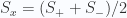
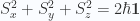
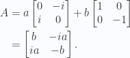
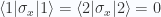
 takes on the values of the total spin for the (possibly composite) spin operator. Thinking about the spin operators in their matrix representation, it’s not obvious to me that we can just add the total spins, so that if
  and
and  are the spin operators for two respective particle, then the total system has a spin operator
  (really
  , since the respective spin operators only act on their respective particles).
 using Pauli matrices.
 eigenvectors


 operators we have

 , we have


 eigenvalue is given by the solution of

 eigenvalue we seek

 is thus given by
 , the two spin
  particles have a combined spin given by


 and
and  eigenvalues respectively as expected.
 , and alter it with the addition of a “small” perturbation
![\begin{aligned}H = H_0 + \lambda H', \qquad \lambda \in [0,1]\end{aligned} \hspace{\stretch{1}}(2.1)](https://s0.wp.com/latex.php?latex=%5Cbegin%7Baligned%7DH+%3D+H_0+%2B+%5Clambda+H%27%2C+%5Cqquad+%5Clambda+%5Cin+%5B0%2C1%5D%5Cend%7Baligned%7D+%5Chspace%7B%5Cstretch%7B1%7D%7D%282.1%29&bg=fafcff&fg=2a2a2a&s=0&c=20201002)


 , this first condition on
  is not much more than a statement that
  .
.  ? For this to be zero we require that both of the following are simultaneously zero


 . We can also expand the
  , which is
 , and
, and  , then this is


 we form (or assume)

 is, and find that it is zero
 , so all the brakets are zero. Utilizing that we have


 . If one supposes that the


 and
and  . The difference is then
![\begin{aligned}H_0 - (a X - i b P)(a X + i b P)=- i a b \left[{X},{P}\right] = - i \frac{\omega}{2} \left[{X},{P}\right]\end{aligned} \hspace{\stretch{1}}(1.3)](https://s0.wp.com/latex.php?latex=%5Cbegin%7Baligned%7DH_0+-+%28a+X+-+i+b+P%29%28a+X+%2B+i+b+P%29%3D-+i+a+b+%5Cleft%5B%7BX%7D%2C%7BP%7D%5Cright%5D++%3D+-+i+%5Cfrac%7B%5Comega%7D%7B2%7D+%5Cleft%5B%7BX%7D%2C%7BP%7D%5Cright%5D%5Cend%7Baligned%7D+%5Chspace%7B%5Cstretch%7B1%7D%7D%281.3%29&bg=fafcff&fg=2a2a2a&s=0&c=20201002)
 value, but what was the sign? Let’s compute so we don’t get it wrong
![\begin{aligned}\left[{x},{ p}\right] \psi&= -i \hbar \left[{x},{\partial_x}\right] \psi \\ &= -i \hbar ( x \partial_x \psi - \partial_x (x \psi) ) \\ &= -i \hbar ( - \psi ) \\ &= i \hbar \psi\end{aligned}](https://s0.wp.com/latex.php?latex=%5Cbegin%7Baligned%7D%5Cleft%5B%7Bx%7D%2C%7B+p%7D%5Cright%5D+%5Cpsi%26%3D+-i+%5Chbar+%5Cleft%5B%7Bx%7D%2C%7B%5Cpartial_x%7D%5Cright%5D+%5Cpsi+%5C%5C+%26%3D+-i+%5Chbar+%28+x+%5Cpartial_x+%5Cpsi+-+%5Cpartial_x+%28x+%5Cpsi%29+%29+%5C%5C+%26%3D+-i+%5Chbar+%28+-+%5Cpsi+%29+%5C%5C+%26%3D+i+%5Chbar+%5Cpsi%5Cend%7Baligned%7D+&bg=fafcff&fg=2a2a2a&s=0&c=20201002)

 produces the form of the Hamiltonian that we used before
 ) and lowering (
 ) operators respectively, and written


![\begin{aligned}\left[{a},{a^\dagger}\right] = 1.\end{aligned} \hspace{\stretch{1}}(1.12)](https://s0.wp.com/latex.php?latex=%5Cbegin%7Baligned%7D%5Cleft%5B%7Ba%7D%2C%7Ba%5E%5Cdagger%7D%5Cright%5D+%3D+1.%5Cend%7Baligned%7D+%5Chspace%7B%5Cstretch%7B1%7D%7D%281.12%29&bg=fafcff&fg=2a2a2a&s=0&c=20201002)
 of the form

 is an eigenstate of
  .
.
 is also an eigenstate of
  .
. has a lower bound of zero) then the state
  for which the energy is the lowest when operated on by


 where up to this point


 and
and  . Recall that
  . This implies that the eigenstates
  are proportional


 operator
 for
for  .
.


 is thus
 .
.

![\begin{aligned}\left[{b},{b^\dagger}\right] = 1,\end{aligned} \hspace{\stretch{1}}(1.32)](https://s0.wp.com/latex.php?latex=%5Cbegin%7Baligned%7D%5Cleft%5B%7Bb%7D%2C%7Bb%5E%5Cdagger%7D%5Cright%5D+%3D+1%2C%5Cend%7Baligned%7D+%5Chspace%7B%5Cstretch%7B1%7D%7D%281.32%29&bg=fafcff&fg=2a2a2a&s=0&c=20201002)

 operator

 we have

 is a real valued function defined in terms of Lagueere polynomials. Working with the expectation of the
 dependence in
  is
is  we can perform the
  integration directly, which is
 expectation which is

 expectation is a slightly different story. There we have
![\begin{aligned}u &= \cos\theta \\ \sin\theta d\theta &= - d(\cos\theta) = -du \\ u &\in [1, -1],\end{aligned} \hspace{\stretch{1}}(2.42)](https://s0.wp.com/latex.php?latex=%5Cbegin%7Baligned%7Du+%26%3D+%5Ccos%5Ctheta+%5C%5C+%5Csin%5Ctheta+d%5Ctheta+%26%3D+-+d%28%5Ccos%5Ctheta%29+%3D+-du+%5C%5C+u+%26%5Cin+%5B1%2C+-1%5D%2C%5Cend%7Baligned%7D+%5Chspace%7B%5Cstretch%7B1%7D%7D%282.42%29&bg=fafcff&fg=2a2a2a&s=0&c=20201002)

 ), over a symmetric interval, so the end result is zero, completing the problem.
 for each component of angular momentum
  , if
, if  is in fact only a function of
  .
. in position space. For that matrix element, we can proceed to insert complete states, and reduce the problem to a question of wavefunctions. That is
 we have
 with the antisymmetric tensor
  so this is zero for all
 ![i \in [1,3]](https://s0.wp.com/latex.php?latex=i+%5Cin+%5B1%2C3%5D&bg=fafcff&fg=2a2a2a&s=0&c=20201002) .
.


 , this is also the general form of the solution.

 do we have
 (one of which is naturally zero due to the singular nature of the matrix).

 and
and  are zero. This allows for the spectral decomposition


 , the unit vector that lies in the direction of the magnetic field, we have
 as are the differential solutions
  . This leaves us with
 in terms of the direction cosines
  of the magnetic field vector

 , perhaps of the following form


 , and
, and  , so the exponentials reduce this nicely to just
 measurement outcomes.
 values, from the operation
  . So, given this initial state, there are really two outcomes that are possible, since we have two distinct eigenvalues. These are
  and
and  , and
, and  respectively.
 (ie: the absolute square of this value). That is
 , and the probability of this is then just
  . On the exam, I think I listed probabilities for three outcomes, with values
  respectively, but in retrospect that seems blatently wrong.
 measurement outcomes.
 contributions before the measurement, the eigenvalues that can be observed for the
  respectively.
 case, our probability is
  , leaving
  as the probability for measurement of the
  (
( kets. That is
 contribution, and would be
 (, and the resulting state has a
  component, and the other is after the
  component.
 is the parity operator, defined by
  , where
  is the eigenket of the position operator
  is the momentum operator conjugate to
  .
.![{\langle {-x'} \rvert} \left[{\Pi},{P}\right] {\lvert {x} \rangle}](https://s0.wp.com/latex.php?latex=%7B%5Clangle+%7B-x%27%7D+%5Crvert%7D+%5Cleft%5B%7B%5CPi%7D%2C%7BP%7D%5Cright%5D+%7B%5Clvert+%7Bx%7D+%5Crangle%7D&bg=fafcff&fg=2a2a2a&s=0&c=20201002) . This is
. This is![\begin{aligned}{\langle {-x'} \rvert} \left[{\Pi},{P}\right] {\lvert {x} \rangle}&={\langle {-x'} \rvert} \Pi P - P \Pi {\lvert {x} \rangle} \\ &={\langle {-x'} \rvert} \Pi P {\lvert {x} \rangle} - {\langle {-x} \rvert} P \Pi {\lvert {x} \rangle} \\ &={\langle {x'} \rvert} P {\lvert {x} \rangle} - {\langle {-x} \rvert} P {\lvert {-x} \rangle} \\ &=- i \hbar \left(\delta(x'-x) \frac{\partial {}}{\partial {x}}-\underbrace{\delta(-x -(-x'))}_{= \delta(x'-x) = \delta(x-x')} \frac{\partial {}}{\partial {-x}}\right) \\ &=- 2 i \hbar \delta(x'-x) \frac{\partial {}}{\partial {x}} \\ &=2 {\langle {x'} \rvert} P {\lvert {x} \rangle} \\ &=2 {\langle {-x'} \rvert} \Pi P {\lvert {x} \rangle} \\ \end{aligned}](https://s0.wp.com/latex.php?latex=%5Cbegin%7Baligned%7D%7B%5Clangle+%7B-x%27%7D+%5Crvert%7D+%5Cleft%5B%7B%5CPi%7D%2C%7BP%7D%5Cright%5D+%7B%5Clvert+%7Bx%7D+%5Crangle%7D%26%3D%7B%5Clangle+%7B-x%27%7D+%5Crvert%7D+%5CPi+P+-+P+%5CPi+%7B%5Clvert+%7Bx%7D+%5Crangle%7D+%5C%5C+%26%3D%7B%5Clangle+%7B-x%27%7D+%5Crvert%7D+%5CPi+P+%7B%5Clvert+%7Bx%7D+%5Crangle%7D+-+%7B%5Clangle+%7B-x%7D+%5Crvert%7D+P+%5CPi+%7B%5Clvert+%7Bx%7D+%5Crangle%7D+%5C%5C+%26%3D%7B%5Clangle+%7Bx%27%7D+%5Crvert%7D+P+%7B%5Clvert+%7Bx%7D+%5Crangle%7D+-+%7B%5Clangle+%7B-x%7D+%5Crvert%7D+P+%7B%5Clvert+%7B-x%7D+%5Crangle%7D+%5C%5C+%26%3D-+i+%5Chbar+%5Cleft%28%5Cdelta%28x%27-x%29+%5Cfrac%7B%5Cpartial+%7B%7D%7D%7B%5Cpartial+%7Bx%7D%7D-%5Cunderbrace%7B%5Cdelta%28-x+-%28-x%27%29%29%7D_%7B%3D+%5Cdelta%28x%27-x%29+%3D+%5Cdelta%28x-x%27%29%7D+%5Cfrac%7B%5Cpartial+%7B%7D%7D%7B%5Cpartial+%7B-x%7D%7D%5Cright%29+%5C%5C+%26%3D-+2+i+%5Chbar+%5Cdelta%28x%27-x%29+%5Cfrac%7B%5Cpartial+%7B%7D%7D%7B%5Cpartial+%7Bx%7D%7D+%5C%5C+%26%3D2+%7B%5Clangle+%7Bx%27%7D+%5Crvert%7D+P+%7B%5Clvert+%7Bx%7D+%5Crangle%7D+%5C%5C+%26%3D2+%7B%5Clangle+%7B-x%27%7D+%5Crvert%7D+%5CPi+P+%7B%5Clvert+%7Bx%7D+%5Crangle%7D+%5C%5C+%5Cend%7Baligned%7D+&bg=fafcff&fg=2a2a2a&s=0&c=20201002)

 and
and 


 ,
,
 just before the measurement is made?


 an
an  right after the measurement?
 is an eigenstate of


 ?
?

 will be nonvanishing? Justify your answer.
 can be expressed as
 .
.
 , and for
  , and these terms vanish. Our expectation value for
  axis.
axis. , where
  is a unitary operator, prove
  .
.


 ) of an operator is the product of all its eigenvectors.


 are those of
  .
.
 .
.
 . Now assume that
  so that
 , and expand the LHS using 3.27 for
 , and rearrange. This gives us

 . The homogeneous equation has the solution
  , so for the complete equation we assume a solution
 , we produce a LDE of

 , so our solution for 3.29 is
 . It is also unnormalizable since we require
  for any
  . Since
  , we must also have
  , completing the exercise.
 . Suppose that the Hamiltonian for this system is given by
 and
and  using these eigenvectors.

 , we get
 . Our normalized eigenvectors are found to be
 and
and  , we then have


 are required. These are


 is
is  . Find an expression for the state at some later time
  ,
,  .
. follows from 3.44
 , is measured for this system. What is the probabilbity that, at time
  , the result
  . For the positive eigenvalue we can also compute the eigenstate to be


 . I’d attempted a rough sketch of this on paper, but won’t bother scanning it here or describing it further.
 .
. and
and 


 or
or  . When I did this on paper originally I got a different answer for this sum, but looking at it now, I can’t see how I managed to get that answer (it had no factors of
  in the result as the one above does).
 and so on.
 and
and  for arbitrary
 is proportional to
 we have

 the system is prepared in the state
 that a particle would be found within
  of
of  and ended up in position
  , and the probability of being within an interval
  , surrounding the point
 , this is just the squared amplitude itself evaluated at the point


 at that time.

 , so we must only expand the cross terms, but those are just
  . This leaves

 , and
, and  , so we see the last two terms are zero. The first two we can evaluate using our previous result 3.54 which was
  . This leaves
 , we have
 so that the Hamiltonian becomes
 ?
? , corresponds to an observation of state
  , after an initial observation of


 for spin 1 in the representation in which
  are diagonal.
 . If, like angular momentum, we assume that we have for


 have not been considered. Do those have any physical interpretation?
 and
and  indirectly. We find
![\begin{aligned}\left[{S_{+}},{S_{-}}\right] &= 2 \hbar S_z \\ \left[{S_{+}},{S_{z}}\right] &= -\hbar S_{+} \\ \left[{S_{-}},{S_{z}}\right] &= \hbar S_{-}.\end{aligned} \hspace{\stretch{1}}(3.8)](https://s0.wp.com/latex.php?latex=%5Cbegin%7Baligned%7D%5Cleft%5B%7BS_%7B%2B%7D%7D%2C%7BS_%7B-%7D%7D%5Cright%5D+%26%3D+2+%5Chbar+S_z+%5C%5C+%5Cleft%5B%7BS_%7B%2B%7D%7D%2C%7BS_%7Bz%7D%7D%5Cright%5D+%26%3D+-%5Chbar+S_%7B%2B%7D+%5C%5C+%5Cleft%5B%7BS_%7B-%7D%7D%2C%7BS_%7Bz%7D%7D%5Cright%5D+%26%3D+%5Chbar+S_%7B-%7D.%5Cend%7Baligned%7D+%5Chspace%7B%5Cstretch%7B1%7D%7D%283.8%29&bg=fafcff&fg=2a2a2a&s=0&c=20201002)
![\left[{S_{z}},{S_{+}}\right]/\hbar = S_{+}](https://s0.wp.com/latex.php?latex=%5Cleft%5B%7BS_%7Bz%7D%7D%2C%7BS_%7B%2B%7D%7D%5Cright%5D%2F%5Chbar+%3D+S_%7B%2B%7D&bg=fafcff&fg=2a2a2a&s=0&c=20201002) , we find
, we find
![\left[{S_{+}},{S_{-}}\right] = 2 \hbar S_z](https://s0.wp.com/latex.php?latex=%5Cleft%5B%7BS_%7B%2B%7D%7D%2C%7BS_%7B-%7D%7D%5Cright%5D+%3D+2+%5Chbar+S_z&bg=fafcff&fg=2a2a2a&s=0&c=20201002) , we find
, we find
 . We could probably pick any
 , and
, and  , but assuming we have no reason for a non-zero phase we try
 , and
, and  , we finally have
 , as expected.
 . Call the eigenstates
  , and determine the probabilities that they will correspond to
  .
.
 we get

 . Now we can call these
  . This corresponds to the eigenvalue of
  being
being  ”.
”. ?
?
 . At the point when the x component spin is observed to be


 , this is
 and
and  with Cramer’s rule, yielding
 and
and  that are probabilities, and after a bit of algebra we find that those are
 (measuring a spin 1 value for


 of measuring a spin 1 value for
  (ie: in the states
  gives a biased prediction of the state of the state
  , just like two orthogonal vectors under the Clifford product.
 instead of
  to eliminate the
  factors. Before considering the expectation values in the arbitrary spin orientation, let’s consider just the expectation values for

 , where
  was a unit vector, and this seems similar. Let’s now consider the arbitrarily oriented spin vector
  , and look at its expectation value.
 as the the rotated image of
  by an azimuthal angle

 projections of this operator
 is a unit norm operator, we find that the expectation values of the coordinates of
  , where the spin is oriented in the
  plane. That gives us

 is true).
 , so that the spin is in the
 . Write
 with respect to the z-axis is
 .
.


 is
is
 case.
case. , for a spin
 ![[S_i]](https://s0.wp.com/latex.php?latex=%5BS_i%5D&bg=fafcff&fg=2a2a2a&s=0&c=20201002) where
where  .
.
![\begin{aligned}[S] = \left\langle{{S}}\right\rangle_{av} &= w_{+} {\langle {+} \rvert} S {\lvert {+} \rangle} +w_{-} {\langle {-} \rvert} S {\lvert {-} \rangle} \\ &= \frac{\hbar}{2}( w_{+} -w_{-} ) \\ &= \frac{\hbar}{2}( w_{+} -(1 - w_{+}) ) \\ &= \hbar w_{+} - \frac{1}{{2}}\end{aligned}](https://s0.wp.com/latex.php?latex=%5Cbegin%7Baligned%7D%5BS%5D+%3D+%5Cleft%5Clangle%7B%7BS%7D%7D%5Cright%5Crangle_%7Bav%7D+%26%3D+w_%7B%2B%7D+%7B%5Clangle+%7B%2B%7D+%5Crvert%7D+S+%7B%5Clvert+%7B%2B%7D+%5Crangle%7D+%2Bw_%7B-%7D+%7B%5Clangle+%7B-%7D+%5Crvert%7D+S+%7B%5Clvert+%7B-%7D+%5Crangle%7D+%5C%5C+%26%3D+%5Cfrac%7B%5Chbar%7D%7B2%7D%28+w_%7B%2B%7D+-w_%7B-%7D+%29+%5C%5C+%26%3D+%5Cfrac%7B%5Chbar%7D%7B2%7D%28+w_%7B%2B%7D+-%281+-+w_%7B%2B%7D%29+%29+%5C%5C+%26%3D+%5Chbar+w_%7B%2B%7D+-+%5Cfrac%7B1%7D%7B%7B2%7D%7D%5Cend%7Baligned%7D+&bg=fafcff&fg=2a2a2a&s=0&c=20201002)
![\begin{aligned}w_{+} = \frac{1}{{\hbar}} [S] + \frac{1}{{2}}\end{aligned}](https://s0.wp.com/latex.php?latex=%5Cbegin%7Baligned%7Dw_%7B%2B%7D+%3D+%5Cfrac%7B1%7D%7B%7B%5Chbar%7D%7D+%5BS%5D+%2B+%5Cfrac%7B1%7D%7B%7B2%7D%7D%5Cend%7Baligned%7D+&bg=fafcff&fg=2a2a2a&s=0&c=20201002)
![\begin{aligned}\rho &=\frac{1}{{2}} ( {\lvert {+} \rangle}{\langle {+} \rvert} +{\lvert {-} \rangle}{\langle {-} \rvert} )+\frac{1}{{\hbar}} [S] ({\lvert {+} \rangle}{\langle {+} \rvert} -{\lvert {+} \rangle}{\langle {+} \rvert}) \\ &=\frac{1}{{2}} I+\frac{1}{{\hbar}} [S] ({\lvert {+} \rangle}{\langle {+} \rvert} -{\lvert {+} \rangle}{\langle {+} \rvert}) \\ \end{aligned}](https://s0.wp.com/latex.php?latex=%5Cbegin%7Baligned%7D%5Crho+%26%3D%5Cfrac%7B1%7D%7B%7B2%7D%7D+%28+%7B%5Clvert+%7B%2B%7D+%5Crangle%7D%7B%5Clangle+%7B%2B%7D+%5Crvert%7D+%2B%7B%5Clvert+%7B-%7D+%5Crangle%7D%7B%5Clangle+%7B-%7D+%5Crvert%7D+%29%2B%5Cfrac%7B1%7D%7B%7B%5Chbar%7D%7D+%5BS%5D+%28%7B%5Clvert+%7B%2B%7D+%5Crangle%7D%7B%5Clangle+%7B%2B%7D+%5Crvert%7D+-%7B%5Clvert+%7B%2B%7D+%5Crangle%7D%7B%5Clangle+%7B%2B%7D+%5Crvert%7D%29+%5C%5C+%26%3D%5Cfrac%7B1%7D%7B%7B2%7D%7D+I%2B%5Cfrac%7B1%7D%7B%7B%5Chbar%7D%7D+%5BS%5D+%28%7B%5Clvert+%7B%2B%7D+%5Crangle%7D%7B%5Clangle+%7B%2B%7D+%5Crvert%7D+-%7B%5Clvert+%7B%2B%7D+%5Crangle%7D%7B%5Clangle+%7B%2B%7D+%5Crvert%7D%29+%5C%5C+%5Cend%7Baligned%7D+&bg=fafcff&fg=2a2a2a&s=0&c=20201002)

![\begin{aligned}\rho =\frac{1}{{2}} I+\frac{1}{{\hbar}} [S_i] \sigma_i=\frac{1}{{2}} (I + [\sigma_i] \sigma_i )\end{aligned}](https://s0.wp.com/latex.php?latex=%5Cbegin%7Baligned%7D%5Crho+%3D%5Cfrac%7B1%7D%7B%7B2%7D%7D+I%2B%5Cfrac%7B1%7D%7B%7B%5Chbar%7D%7D+%5BS_i%5D+%5Csigma_i%3D%5Cfrac%7B1%7D%7B%7B2%7D%7D+%28I+%2B+%5B%5Csigma_i%5D+%5Csigma_i+%29%5Cend%7Baligned%7D+&bg=fafcff&fg=2a2a2a&s=0&c=20201002)
![\mathbf{P}_i = [\sigma_i] \mathbf{e}_i](https://s0.wp.com/latex.php?latex=%5Cmathbf%7BP%7D_i+%3D+%5B%5Csigma_i%5D+%5Cmathbf%7Be%7D_i&bg=fafcff&fg=2a2a2a&s=0&c=20201002) , for any of the directions
, for any of the directions  we can write
 , and the individual weights
  , and
, and  , but we see here that this
  factor can be written exclusively in terms of the ensemble average. Actually, this is also a result in the text, down in (5.113), but we see it here in a more concrete form having picked specific spin directions.
 , determine the time evolution operator as a 2 x 2 matrix. If a state at


 , and
, and  , we have

 as expected.
 , we have


 for
for  and
and  , and
, and  .)
.) , when simplified, has a term proportional to
  .
.
 , we have
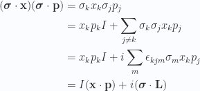
![\begin{aligned}\left[{ \boldsymbol{\sigma} \cdot \mathbf{p}},{V(r)}\right]&=- \frac{i \hbar}{r} \frac{\partial {V(r)}}{\partial {r}} (\boldsymbol{\sigma} \cdot \mathbf{x}) \end{aligned} \hspace{\stretch{1}}(3.72)](https://s0.wp.com/latex.php?latex=%5Cbegin%7Baligned%7D%5Cleft%5B%7B+%5Cboldsymbol%7B%5Csigma%7D+%5Ccdot+%5Cmathbf%7Bp%7D%7D%2C%7BV%28r%29%7D%5Cright%5D%26%3D-+%5Cfrac%7Bi+%5Chbar%7D%7Br%7D+%5Cfrac%7B%5Cpartial+%7BV%28r%29%7D%7D%7B%5Cpartial+%7Br%7D%7D+%28%5Cboldsymbol%7B%5Csigma%7D+%5Ccdot+%5Cmathbf%7Bx%7D%29+%5Cend%7Baligned%7D+%5Chspace%7B%5Cstretch%7B1%7D%7D%283.72%29&bg=fafcff&fg=2a2a2a&s=0&c=20201002)

 into symmetric and antisymmetric components, we should have in the second term our
![\begin{aligned}(\boldsymbol{\sigma} \cdot \mathbf{x}) (\boldsymbol{\sigma} \cdot \mathbf{p} )=\frac{1}{{2}} \left\{{\boldsymbol{\sigma} \cdot \mathbf{x}},{\boldsymbol{\sigma} \cdot \mathbf{p}}\right\}+\frac{1}{{2}} \left[{\boldsymbol{\sigma} \cdot \mathbf{x}},{\boldsymbol{\sigma} \cdot \mathbf{p}}\right]\end{aligned} \hspace{\stretch{1}}(3.74)](https://s0.wp.com/latex.php?latex=%5Cbegin%7Baligned%7D%28%5Cboldsymbol%7B%5Csigma%7D+%5Ccdot+%5Cmathbf%7Bx%7D%29+%28%5Cboldsymbol%7B%5Csigma%7D+%5Ccdot+%5Cmathbf%7Bp%7D+%29%3D%5Cfrac%7B1%7D%7B%7B2%7D%7D+%5Cleft%5C%7B%7B%5Cboldsymbol%7B%5Csigma%7D+%5Ccdot+%5Cmathbf%7Bx%7D%7D%2C%7B%5Cboldsymbol%7B%5Csigma%7D+%5Ccdot+%5Cmathbf%7Bp%7D%7D%5Cright%5C%7D%2B%5Cfrac%7B1%7D%7B%7B2%7D%7D+%5Cleft%5B%7B%5Cboldsymbol%7B%5Csigma%7D+%5Ccdot+%5Cmathbf%7Bx%7D%7D%2C%7B%5Cboldsymbol%7B%5Csigma%7D+%5Ccdot+%5Cmathbf%7Bp%7D%7D%5Cright%5D%5Cend%7Baligned%7D+%5Chspace%7B%5Cstretch%7B1%7D%7D%283.74%29&bg=fafcff&fg=2a2a2a&s=0&c=20201002)
![\boldsymbol{\sigma} \cdot \mathbf{L} \propto \left[{\boldsymbol{\sigma} \cdot \mathbf{x}},{\boldsymbol{\sigma} \cdot \mathbf{p}}\right]](https://s0.wp.com/latex.php?latex=%5Cboldsymbol%7B%5Csigma%7D+%5Ccdot+%5Cmathbf%7BL%7D+%5Cpropto+%5Cleft%5B%7B%5Cboldsymbol%7B%5Csigma%7D+%5Ccdot+%5Cmathbf%7Bx%7D%7D%2C%7B%5Cboldsymbol%7B%5Csigma%7D+%5Ccdot+%5Cmathbf%7Bp%7D%7D%5Cright%5D&bg=fafcff&fg=2a2a2a&s=0&c=20201002) . Alternately in components
. Alternately in components