My dad asks
” I’ve googled some data about “c”, the speed of light, but found really no data about why this is the speed limit that a particle can travel. It is just stated to be so but no allusions ( except Einstein’s smoke and mirrors) were indicated as to why this was the case.”
Here was my attempt at answering. I liked it and share it here.
For light itself, this is an observed quality. Light in vacuum hasn’t been observed travelling at any other velocity. There have been lots of experiments attempting to show otherwise, and none of them worked. Where people get hung up is that they think of light as a thrown object, like a ball tossed out of a car window. If you are (the passenger) in a convertible (let’s say this is a Porsche for fun) that is zipping down the street at 90mph, and toss a baseball at 50mph somebody on the sidewalk will see that ball travelling at 140mph. If you through it backwards, an observer will see it moving at just 40mph. We have lots of experience with “addition of velocities like this”.
With light, something that’s already tricky to measure because it is so fast, we don’t have a lot of experience. However, when an experiment like this is done carefully, from a fast moving object, it is carries a light pointing in its direction of motion, an observer will see the light emitted go at the speed of light, regardless of the speed of the object. If you imagine a rocket that’s moving at 1/2 the speed of light itself, it’s headlight emits light that seen to travel at c (not 1.5c), and it’s taillight is seen to emit light that travels at c (not 0.5c). This is very different from the ball and the car example.
The way that I think of this is that the light was not, then is. At that point of creation, it moves at speed c, but this motion is never associated with the speed of any nearby objects (ie. this light at the point of creation was never carried by the object that’s travelling in its vicinity).
Since we have this phenomena that always appears to have a fixed velocity, we can use it as both a measuring stick and as a clock. If light is bounced off of a mirror and returns (assuming that the delay for the interaction with the mirror is negligible), then if we’ve counted out the distance to the mirror (say d), then we would know that an interval of time 2d/c has passed. Similarly, if clocks are synchronized at two points in space, with you standing by one clock and your buddy standing by another with an agreement to turn on his light at 12:00, and you observe that his light signal gets to you at 12:00:000003, then the distance between you is .0003 seconds x c = 90km. The basic idea is that you can use light signals as a mechanism for both time and space depending on what you know.
What Einstein did was argue very carefully that there is no such concept as simultaneity. Events that are simultaneous can be observer dependent and we have to alter the way that we describe time and space to account for this. Light ends up having a place as a measuring stick for this new way of describing time and space. When space and time and motions in space and time are treated carefully, to ensure that notions of time and distance are related to the observer and the observers own motion, there are some interesting consequences.
One of these consequences is that velocities don’t add like the ball and car example. There is a very very small correction required, and if one were to able to measure the speed of the ball thrown forward over the front windshield of the Porsche, you would find that it is actually a tiny bit less than 140mph. That correction gets bigger and bigger, as the speeds of the objects are increased.
If you had a rocket turbocharger on the Porche and was able to launch it into space at .75 c, and then tossed the ball into a turbocharged baseball pitching device that could propel it at 0.5 c, then you’ll see the ball moving at 0.5 c, but an observer will NOT see it moving at 0.75c+0.5c=1.25c. It will actually be observed to travel at less than 1.0 c. There is a lot of math involved and this can be thought of as Smoke and Mirrors if you like (and perhaps justifiably so since it’s not terribly easy math to learn), but again this is something that is backed up by experiment. It takes a lot of care to measure things when interactions happen at such high velocities (velocities that are significant factions of the speed of light), but when you do velocities are never seen to add to more than the speed of light, regardless of the motion of the observed interactions. This is why in a very real way: it has never been observed to be otherwise.
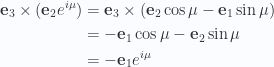
 moving in a circle of radius
  at constant angular frequency
  .
.


 and
and  for any
  .
. to select the scalar part of a multivector (or with the Pauli matrices, the portion proportional to the identity matrix).


 , and having a peek back at 1.4, our potentials are now solved for
 is only specified implicitly, according to


 from 1.14, this is
 what do we have?


 becomes constant (in my exam attempt I somehow fudged this to get what I wanted for the
  case, but that must have been wrong, and was the result of rushed work).


 )).
)).


 relative to
  has four momentum


 ). That gives (and this time keeping my cross terms)
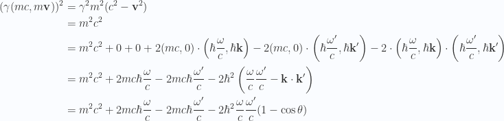


 .
.

 and
and  need
need  , and
, and 


 .
.


 .
. , since the denominator is smallest (
 is not small. This is strongly


 perpendicular to that, strongest when charge is moving fast.


 is called the radiated power.

 replacing the usual
  .
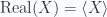
. and another point, say
  motivates the inner product between two points in this representation


 , but we are free to pick any other basis should we choose. In particular, if we rotate our basis counterclockwise by
  , our new basis, still orthonormal, is
  .
.

 , and
, and  are the (real) coordinates of the point
  in this rotated basis.
 at an arbitrary angle
 coordinates as a check. For the spatial component parallel to the boost direction we have


 is found to be (after a bit of work)

 (190-193); the “Darwin Lagrangian. and Hamiltonian for a system of nonrelativistic charged particles to order
  – radiation damping, the limitations of classical electrodynamics, and the relevant time/length/energy scales.
![m_a, q_a ; a \in [1, N]](https://s0.wp.com/latex.php?latex=m_a%2C+q_a+%3B+a+%5Cin+%5B1%2C+N%5D&bg=fafcff&fg=2a2a2a&s=0&c=20201002) closed system and nonrelativistic,
closed system and nonrelativistic,  . In this case we can incorporate EM effects in a Largrangian ONLY involving particles (EM field not a dynamical DOF). In general case, this works to
  , because at
  system radiation effects occur.
 because of specific symmetries in such a system.


 obvious problem due to radiation (system not closed). We’ll incorporate radiation via a function term in the EOM


 we have


 . The first integral above is zero since the derivative of
  is also periodic, and vanishes when integrated over the interval.


 is the “classical radius” of the electron. In our frictional term we have
  , the time for light to cross the classical radius of the electron.
 . Then we have


 , but those examples are harder to find (see: [2]).
 ) should be taken seriously only if it is small compared to the first two terms.
 is the Maxwell stress tensor for the incident wave, and
  is the Maxwell stress tensor for the reflected wave, and
  is normal to the wall.
 component of the field momentum
 , and
, and  is the outwards unit normal to the surface. This is the rate of change of momentum for the field, the force on the field. For the force on the wall per unit area, we wish to invert this, giving


 and
and  respectively.


 . I don’t see where that comes from, since the propagation directions are difference for the incident and the reflected waves.


 and
and  are the total EM fields.


 and
and  . Are these parallel to the wall or parallel to the normal to the wall. It turns out that this appears to mean parallel to the normal. We can see this by direct calculation


 place
place  we have


 )
)


 ,
,  reflected in a plane, separated by distance
 .
.


