[Click here for a PDF of this post with nicer formatting (especially if my latex to wordpress script has left FORMULA DOES NOT PARSE errors.)]
Motivation
We’re discussing specific forms to systems of coupled linear differential equations, such as a loop of “spring” connected masses (i.e. atoms interacting with harmonic oscillator potentials) as sketched in fig. 1.1.

Fig 1.1: Three springs loop
Instead of assuming a solution, let’s see how far we can get attacking this problem systematically.
Matrix methods
Suppose that we have a set of  masses constrained to a circle interacting with harmonic potentials. The Lagrangian for such a system (using modulo indexing) is

The force equations follow directly from the Euler-Lagrange equations

For the simple three particle system depicted above, this is

with equations of motion

Let’s partially non-dimensionalize this. First introduce average mass  and spring constants
  , and rearrange slightly

With


Our system takes the form

We can at least theoretically solve this in a simple fashion if we first convert it to a first order system. We can do that by augmenting our vector of displacements with their first derivatives

So that

Now the solution is conceptually trivial

We are however, faced with the task of exponentiating the matrix  . All the powers of this matrix will be required, but they turn out to be easy to calculate


allowing us to write out the matrix exponential

Case I: No zero eigenvalues
Provided that  has no zero eigenvalues, we could factor this as

This initially leads us to believe the following, but we’ll find out that the three springs interaction matrix does have a zero eigenvalue, and we’ll have to be more careful. If there were any such interaction matrices that did not have such a zero we could simply write

This is

The solution, written out is

so that

As a check differentiation twice shows that this is in fact the general solution, since we have

and

Observe that this solution is a general solution to second order constant coefficient linear systems of the form we have in eq. 1.5. However, to make it meaningful we do have the additional computational task of performing an eigensystem decomposition of the matrix . We expect negative eigenvalues that will give us oscillatory solutions (ie: the matrix square roots will have imaginary eigenvalues).
Example: An example diagonalization to try things out
{example:threeSpringLoop:1}{
Let’s do that diagonalization for the simplest of the three springs system as an example, with  and
and  , so that we have

A orthonormal eigensystem for is

With

We have

We also find that and its root are intimately related in a surprising way

We also see, unfortunately that has a zero eigenvalue, so we can’t compute  . We’ll have to back and up and start again differently.
}
Case II: allowing for zero eigenvalues
Now that we realize we have to deal with zero eigenvalues, a different approach suggests itself. Instead of reducing our system using a Hamiltonian transformation to a first order system, let’s utilize that diagonalization directly. Our system is

where ![D = [ \lambda_i \delta_{ij} ]](https://s0.wp.com/latex.php?latex=D+%3D+%5B+%5Clambda_i+%5Cdelta_%7Bij%7D+%5D&bg=fafcff&fg=2a2a2a&s=0&c=20201002) and
and

Let

so that our system is just

or

This is equations, each decoupled and solvable by inspection. Suppose we group the eigenvalues into sets  . Our solution is then

Transforming back to lattice coordinates using  , we have

We see that the zero eigenvalues integration terms have no contribution to the lattice coordinates, since  , for all
  .
.
If ![U = [ \mathbf{e}_i ]](https://s0.wp.com/latex.php?latex=U+%3D+%5B+%5Cmathbf%7Be%7D_i+%5D&bg=fafcff&fg=2a2a2a&s=0&c=20201002) are a set of not necessarily orthonormal eigenvectors for , then the vectors
are a set of not necessarily orthonormal eigenvectors for , then the vectors  , where
  are the reciprocal frame vectors. These can be extracted from
 ![U^{-1} = [ \mathbf{f}_i ]^\text{T}](https://s0.wp.com/latex.php?latex=U%5E%7B-1%7D+%3D+%5B+%5Cmathbf%7Bf%7D_i+%5D%5E%5Ctext%7BT%7D&bg=fafcff&fg=2a2a2a&s=0&c=20201002) (i.e., the rows of
(i.e., the rows of  ). Taking dot products between with
  and
and  , provides us with the unknown coefficients

Supposing that we constrain ourself to looking at just the oscillatory solutions (i.e. the lattice does not shake itself to pieces), then we have

Eigenvectors for eigenvalues that were degenerate have been explicitly enumerated here, something previously implied. Observe that the dot products of the form  have been put into projector operator form to group terms more nicely. The solution can be thought of as a weighted projector operator working as a time evolution operator from the initial state.
Example: Our example interaction revisited
{example:threeSpringLoop:2}{
Recall that we had an orthonormal basis for the  eigensubspace for the interaction example of eq. 1.20 again, so
  . We can sum
  to find

The leading matrix is an orthonormal projector of the initial conditions onto the eigen subspace for  . Observe that this is proportional to itself, scaled by the square of the non-zero eigenvalue of
  . From this we can confirm by inspection that this is a solution to
  , as desired.
}
Fourier transform methods
Let’s now try another item from our usual toolbox on these sorts of second order systems, the Fourier transform. For a one variable function of time let’s write the transform pair as


One mass harmonic oscillator
The simplest second order system is that of the harmonic oscillator

Application of the transform gives

We clearly have a constraint that is a function of frequency, but one that has to hold for all time. Let’s transform this constraint to the frequency domain to consider that constraint independent of time.

How do we make sense of this?
Since  is an integration variable, we can’t just mandate that it equals the constant driving frequency
  . It’s clear that we require a constraint on the transform
  as well. As a trial solution, imagine that
 latex \left\lvert {\omega – \pm \omega_\circ} \right\rvert < \omega_{\text{cutoff}}$} \\ 0 & \quad \mbox{otherwise}\end{array}\right.\end{aligned} \hspace{\stretch{1}}(1.0.35.35)$
This gives us

Now it is clear that we can satisfy our constraint only if the interval ![[\pm \omega_\circ -\omega_{\text{cutoff}}, \pm \omega_\circ + \omega_{\text{cutoff}}]](https://s0.wp.com/latex.php?latex=%5B%5Cpm+%5Comega_%5Ccirc+-%5Comega_%7B%5Ctext%7Bcutoff%7D%7D%2C+%5Cpm+%5Comega_%5Ccirc+%2B+%5Comega_%7B%5Ctext%7Bcutoff%7D%7D%5D&bg=fafcff&fg=2a2a2a&s=0&c=20201002) is made infinitesimal. Specifically, we require both a
is made infinitesimal. Specifically, we require both a  constraint and that the transform have a delta function nature. That is

Substitution back into our transform gives

We can verify quickly that this satisfies our harmonic equation  .
.
Two mass harmonic oscillator
Having applied the transform technique to the very simplest second order system, we can now consider the next more complex system, that of two harmonically interacting masses (i.e. two masses on a frictionless spring).
F1
Our system is described by

and the pair of Euler-Lagrange equations

The equations of motion are

Let

Insertion of these transform pairs into our equations of motion produces a pair of simultaneous integral equations to solve

As with the single spring case, we can decouple these equations with an inverse transformation operation  , which gives us (after dropping primes)

Taking determinants gives us the constraint on the frequency

Introducing a reduced mass

the pair of solutions are

As with the single mass oscillator, we require the functions  to also be expressed as delta functions. The frequency constraint and that delta function requirement together can be expressed, for
  as
as

With a transformation back to time domain, we have functions of the form

Back insertion of these into the equations of motion, we have

Equality requires identity for all powers of  , or
, or

or  and
and

Observe that

(with a similar alternate result). We can rewrite eq. 1.0.35.35 as

It’s clear that there’s two pairs of linear dependencies here, so the determinant is zero as expected. We can read off the remaining relations. Our undetermined coefficients are given by


Observe that the constant term is not really of interest, since it represents a constant displacement of both atoms (just a change of coordinates).
Check:


Reflection
We’ve seen that we can solve any of these constant coefficient systems exactly using matrix methods, however, these will not be practical for large systems unless we have methods to solve for all the non-zero eigenvalues and their corresponding eigenvectors. With the Fourier transform methods we find that our solutions in the frequency domain is of the form

or in the time domain

We assumed exactly this form of solution in class. The trial solution that we used in class factored out a phase shift from  of the form of
  , but that doesn’t change the underling form of that assumed solution. We have however found a good justification for the trial solution we utilized.


 as in fig. 2.1, where
  .
.


 , as illustrated in fig. 2.2.
 between lattice points indexed
  (located at
  and
and  respectively), and direction cosines for the equilibrium direction vector between those points given by


 . Equating both, we have in vector form

 and vertical height is
  .
.

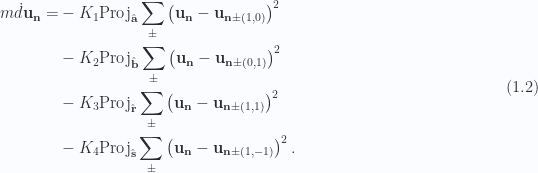
 assume a trial solution of the form


 for the projection operators, this is


 for matrix
 .
.

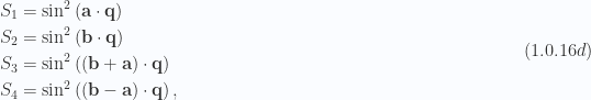
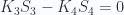
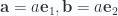
 and
and  projection operators, we can use half angle formulations


 , and
, and  , so
, so


 we can use a linear approximation


 result for the thermal average energy.
 as above. This gives us
 of a system with two states, one at energy
  and one at energy
  . From the free energy, find expressions for the energy and entropy of the system.


 and the susceptibility
  as a function of temperature and magnetic field for the model system of magnetic moments in a magnetic field. The result for the magnetization, found by other means, was
  , where
  is the particle concentration. Find the free energy and express the result as a function only of
  . Show that the susceptibility is
  in the limit
  .
.


 , the cosh term goes to unity, so we have
 , the free energy is
 , where
  is a positive integer or zero, and
  . Show that for a harmonic oscillator the free energy is
 we may expand the argument of the logarithm to obtain
  . From 1.0.16 show that the entropy is
 from the energy. Including it we have


 in the energy of each state just adds a constant factor to the free energy. This will drop out when we compute the entropy. Dropping that factor now that we know why it doesn’t contribute, we can complete the summation, so have, by inspection


 is the conventional symbol for
  . Hint: Use the partition function
  to relate
  to the mean square fluctuation. Also, multiply out the term
  .
.


 to
to 


 in figure (\ref{fig:gaussianWavePacket}).
 , and width proportional to
  .
.
 , in figure (\ref{fig:FTgaussianWavePacket})
 and
and  fixed, and decrease
  . We can formally integrate 3.8

 . However, we can select the small interval
  , and write
 and then develop this, to generate a power series with
  dependence. However, we note that 3.11 is still an exact relation, and if
  is well behaved) we are left with just


 continuously, but very quickly. In effect, we have tightened the spring constant. Note that there are cases in linear optics when you can actually do exactly that.
 is in the ground state of the harmonic oscillator as in figure (\ref{fig:suddenHamiltonianPertubationHO})
 (weakening the “spring”). Professor Sipe gives us a graphical demo of this, by impersonating a constrained wavefunction with his arms, doing weak chicken-flapping of them. Now with the potential weakended, he wiggles and flaps his arms with more freedom and somewhat chaotically. His “wave function” arms are now bouncing around in the new limiting potential (initally over doing it and then bouncing back).


 very slowly.
 write
write

 we can find the “instantaneous” energy eigenstates


 into this

 is also changing very very slowly, but we are not quite there yet. Let’s first split our sum of bra and ket products
 and
and  terms. Looking at just the


 must be purely imaginary. We write
 is real.
 is plotted in figure (\ref{fig:expMinusBetsAbsX})
 , this is plotted in figure (\ref{fig:expMinusBetsAbsXfirstOrderFitting}) and can be seen to match fairly well
 as plotted in figure (\ref{fig:stepFunction}).
 , we have for the derivative of the absolute value function
 , and
, and  derivative for
  . At the origin our
  contributions vanish, and we are left with
 and integrate. Doing so we have
 as zero at the origin.


![\begin{aligned}E[\beta] = \frac{{\langle {\psi} \rvert} H {\lvert {\psi} \rangle}}{\left\langle{{\psi}} \vert {{\psi}}\right\rangle} = \frac{\beta^2 \hbar^2}{2m} + \frac{m \omega^2}{4 \beta^2}.\end{aligned} \hspace{\stretch{1}}(7.20)](https://s0.wp.com/latex.php?latex=%5Cbegin%7Baligned%7DE%5B%5Cbeta%5D+%3D+%5Cfrac%7B%7B%5Clangle+%7B%5Cpsi%7D+%5Crvert%7D+H+%7B%5Clvert+%7B%5Cpsi%7D+%5Crangle%7D%7D%7B%5Cleft%5Clangle%7B%7B%5Cpsi%7D%7D+%5Cvert+%7B%7B%5Cpsi%7D%7D%5Cright%5Crangle%7D+%3D+%5Cfrac%7B%5Cbeta%5E2+%5Chbar%5E2%7D%7B2m%7D+%2B+%5Cfrac%7Bm+%5Comega%5E2%7D%7B4+%5Cbeta%5E2%7D.%5Cend%7Baligned%7D+%5Chspace%7B%5Cstretch%7B1%7D%7D%287.20%29&bg=fafcff&fg=2a2a2a&s=0&c=20201002)
 when
when ![E[\beta]](https://s0.wp.com/latex.php?latex=E%5B%5Cbeta%5D&bg=fafcff&fg=2a2a2a&s=0&c=20201002) is minimized. That is
is minimized. That is


![\begin{aligned}E[\beta_{\text{min}}] = \frac{\hbar \omega}{2} \sqrt{2}\end{aligned} \hspace{\stretch{1}}(7.24)](https://s0.wp.com/latex.php?latex=%5Cbegin%7Baligned%7DE%5B%5Cbeta_%7B%5Ctext%7Bmin%7D%7D%5D+%3D+%5Cfrac%7B%5Chbar+%5Comega%7D%7B2%7D+%5Csqrt%7B2%7D%5Cend%7Baligned%7D+%5Chspace%7B%5Cstretch%7B1%7D%7D%287.24%29&bg=fafcff&fg=2a2a2a&s=0&c=20201002)
 the true ground state energy, but is at least a ball park value. However, to get this result, we have to be very careful to treat our point of singularity. A derivative that we’d call undefined in first year calculus, is not only defined, but required, for this treatment to work!
 . Is the state
 is given by Eq. (9.60),
  , an energy eigenstate of the system? What is probability per unit length for measuring the particle at position
  at
at  ? Explain the physical meaning of the above results.
 ,
,  , and
, and  . With this variable substitution Schr\”{o}dinger’s equation for this harmonic oscillator potential takes the form
 into this to get
 , this isn’t a normalizable wavefunction, and has no physical relevance, unless we set
  .
. latex x < a$} \\ \frac{1}{{2}} K x^2 & \quad \mbox{if $latex a < x b$} \\ \end{array}\right.\end{aligned} \hspace{\stretch{1}}(2.3)$
 , for constant
  . For such a potential, within the harmonic well, a general solution of the form
 values in that situation. For the wave function to be a physically relevant, we require it to be (absolute) square integrable, and must also integrate to unity over the entire interval.
 (that probability is zero in a continuous space), but we can answer the question for the probability that a particle is found in an interval surrounding a specific point at this time. By calculating the average of the probability to find the particle in an interval, and dividing by that interval’s length, we arrive at plausible definition of probability per unit length for an interval surrounding
 latex x = x_0$} =\lim_{\epsilon \rightarrow 0} \frac{1}{{\epsilon}} \int_{x_0 – \epsilon/2}^{x_0 + \epsilon/2} {\left\lvert{ \Psi(x, t_0) }\right\rvert}^2 dx = {\left\lvert{\Psi(x_0, t_0)}\right\rvert}^2\end{aligned} \hspace{\stretch{1}}(2.5)$
 wavefunction 2.1. Since normalization requires
  , that probability density is simply zero (or undefined, depending on one’s point of view).
 coefficients yield unit probability
 , we have
 we have just
 may equal
  (this is true at least up to n=4). If that’s the case, we have for non-mixed states, with even numbered energy quantum numbers, at
  .
.