[Click here for a PDF of this post with nicer formatting (especially if my latex to wordpress script has left FORMULA DOES NOT PARSE errors.)]
Charged particle in a circle.
From the 2008 PHY353 exam, given a particle of charge  moving in a circle of radius
  at constant angular frequency
  .
.
\begin{itemize}
\item Find the Lienard-Wiechert potentials for points on the z-axis.
\item Find the electric and magnetic fields at the center.
\end{itemize}
When I tried this I did it for points not just on the z-axis. It turns out that we also got this question on the exam (but stated slightly differently). Since I’ll not get to see my exam solution again, let’s work through this at a leisurely rate, and see if things look right. The problem as stated in this old practice exam is easier since it doesn’t say to calculate the fields from the four potentials, so there was nothing preventing one from just grinding away and plugging stuff into the Lienard-Wiechert equations for the fields (as I did when I tried it for practice).
The potentials.
Let’s set up our coordinate system in cylindrical coordinates. For the charged particle and the point that we measure the field, with 

Here I’m using the geometric product of vectors (if that’s unfamiliar then just substitute

We can do that since the Pauli matrices also have the same semantics (with a small difference since the geometric square of a unit vector is defined as the unit scalar, whereas the Pauli matrix square is the identity matrix). The semantics we require of this vector product are just  and
and  for any
  .
.
I’ll also be loose with notation and use  to select the scalar part of a multivector (or with the Pauli matrices, the portion proportional to the identity matrix).
Our task is to compute the Lienard-Wiechert potentials. Those are

where

We’ll need (eventually)

and also need our retarded distance vector

From this we have
So

Next we need

So we have

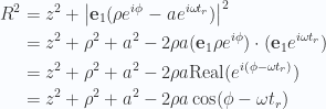
Writing  , and having a peek back at 1.4, our potentials are now solved for

The caveat is that  is only specified implicitly, according to

There doesn’t appear to be much hope of solving for explicitly in closed form.
General fields for this system.
With

the fields are

In there we have

and

Writing this out in coordinates isn’t particularly illuminating, but can be done for completeness without too much trouble

In one sense the problem could be considered solved, since we have all the pieces of the puzzle. The outstanding question is whether or not the resulting mess can be simplified at all. Let’s see if the cross product reduces at all. Using

Perhaps one or more of these dot products can be simplified? One of them does reduce nicely

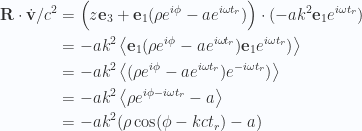
Putting this cross product back together we have
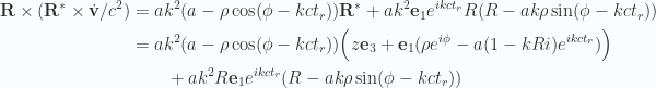
Writing

this can be grouped into similar terms

The electric field pieces can now be collected. Not expanding out the  from 1.14, this is

Along the z-axis where  what do we have?


The magnetic term here looks like it can be reduced a bit.
An approximation near the center.
Unlike the old exam I did, where it didn’t specify that the potentials had to be used to calculate the fields, and the problem was reduced to one of algebraic manipulation, our exam explicitly asked for the potentials to be used to calculate the fields.
There was also the restriction to compute them near the center. Setting so that we are looking only near the z-axis, we have

Now we are set to calculate the electric and magnetic fields directly from these. Observe that we have a spatial dependence in due to the quantities and that will have an effect when we operate with the gradient.
In the exam I’d asked Simon (our TA) if this question was asking for the fields at the origin (ie: in the plane of the charge’s motion in the center) or along the z-axis. He said in the plane. That would simplify things, but perhaps too much since  becomes constant (in my exam attempt I somehow fudged this to get what I wanted for the
  case, but that must have been wrong, and was the result of rushed work).
Let’s now proceed with the field calculation from these potentials

For the electric field we need

and

Putting these together, our electric field near the z-axis is

(another mistake I made on the exam, since I somehow fooled myself into forcing what I knew had to be in the gradient term, despite having essentially a constant scalar potential (having taken  )).
)).
What do we get for the magnetic field. In that case we have

For the direction vectors in the cross products above we have
and

Putting everything, and summarizing results for the fields, we have

The electric field expression above compares well to 1.29. We have the Coulomb term and the radiation term. It is harder to compare the magnetic field to the exact result 1.30 since I did not expand that out.
FIXME: A question to consider. If all this worked should we not also get

However, if I do this check I get

Collision of photon and electron.
I made a dumb error on the exam on this one. I setup the four momentum conservation statement, but then didn’t multiply out the cross terms properly. This led me to incorrectly assume that I had to try doing this the hard way (something akin to what I did on the midterm). Simon later told us in the tutorial the simple way, and that’s all we needed here too. Here’s the setup.
An electron at rest initially has four momentum

where the incoming photon has four momentum

After the collision our electron has some velocity so its four momentum becomes (say)

and our new photon, going off on an angle  relative to
  has four momentum

Our conservation relationship is thus

I squared both sides, but dropped my cross terms, which was just plain wrong, and costly for both time and effort on the exam. What I should have done was just

and then square this (really making contractions of the form  ). That gives (and this time keeping my cross terms)
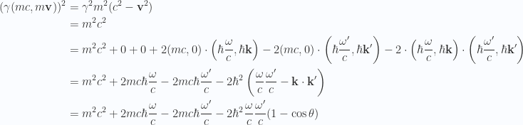
Rearranging a bit we have

or

Pion decay.
The problem above is very much like a midterm problem we had, so there was no justifiable excuse for messing up on it. That midterm problem was to consider the split of a pion at rest into a neutrino (massless) and a muon, and to calculate the energy of the muon. That one also follows the same pattern, a calculation of four momentum conservation, say

Here is the frequency of the massless neutrino. The massless nature is encoded by a four momentum that squares to zero, which follows from  .
.
When I did this problem on the midterm, I perversely put in a scattering angle, instead of recognizing that the particles must scatter at 180 degree directions since spatial momentum components must also be preserved. This and the combination of trying to work in spatial quantities led to a mess and I didn’t get the end result in anything that could be considered tidy.
The simple way to do this is to just rearrange to put the null vector on one side, and then square. This gives us

A final re-arrangement gives us the muon energy

 – radiation damping, the limitations of classical electrodynamics, and the relevant time/length/energy scales.
 .
.
 . For the charge density this is


 term, and now move on to
  . We will write
  as a total derivative
 previously.

 , and then employ integration by parts


 there is a homogeneous electric field felt by all particles, hence every particle feels a “friction” force
 arises in third order term
 is the classical radius of the electron. For periodic motion


 , this approximation is valid.


 and
and  pairs. A theory where the number of particles (electrons and positrons) is NOT fixed anymore is required. An estimate of this frequency, where these effects have to be considered is possible.
 ,
,  . LHC exploration.
 ,
,  , the Compton wavelength of the electron. QED and quantum field theory.
 , Bohr radius. QM, and classical electrodynamics.


 and
and  is then

 , which is


 and
and 


 ? That gives us
 , can be tidied up a bit more, but this won’t be persued here. Instead let’s write out the fields corresponding to the potentials of 1.7 explicitly. We need to calculate
  ,
,  ,
,  , and
, and  . For the acceleration we get


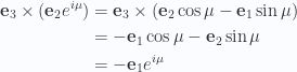
 will rotate in the
  plane, which accounts for the factors of
  in the complex portion of the cross product. The imaginary part has only contributions from the portions of the vectors
  and
and  that are perpendicular to each other, so while the real part of
  measures the colinearity, the imaginary part is a measure of the amount perpendicular.


 and
and  , which kills a number of the terms
 also becomes irrelevant. In that case we have along the z-axis the fields are given by


 here I’d guess I’ve got an algebraic error hiding somewhere?
 , and
, and 


 .
.


 .
. , since the denominator is smallest (


 perpendicular to that, strongest when charge is moving fast.


 is called the radiated power.
 (190-193); the “Darwin Lagrangian. and Hamiltonian for a system of nonrelativistic charged particles to order
 ![m_a, q_a ; a \in [1, N]](https://s0.wp.com/latex.php?latex=m_a%2C+q_a+%3B+a+%5Cin+%5B1%2C+N%5D&bg=fafcff&fg=2a2a2a&s=0&c=20201002) closed system and nonrelativistic,
closed system and nonrelativistic,  . In this case we can incorporate EM effects in a Largrangian ONLY involving particles (EM field not a dynamical DOF). In general case, this works to
  , because at
  system radiation effects occur.
 because of specific symmetries in such a system.


 we have


 . The first integral above is zero since the derivative of
  is also periodic, and vanishes when integrated over the interval.


 , the time for light to cross the classical radius of the electron.
 . Then we have


 , but those examples are harder to find (see: [2]).
 ) should be taken seriously only if it is small compared to the first two terms.
 is the Maxwell stress tensor for the incident wave, and
  is the Maxwell stress tensor for the reflected wave, and
  is normal to the wall.
 component of the field momentum
 , and
, and  is the outwards unit normal to the surface. This is the rate of change of momentum for the field, the force on the field. For the force on the wall per unit area, we wish to invert this, giving


 and
and  respectively.


 . I don’t see where that comes from, since the propagation directions are difference for the incident and the reflected waves.


 and
and  are the total EM fields.


 and
and  . Are these parallel to the wall or parallel to the normal to the wall. It turns out that this appears to mean parallel to the normal. We can see this by direct calculation


 place
place  we have


 )
)


 ,
,  reflected in a plane, separated by distance
 .
.


