[Click here for a PDF of this post with nicer formatting (especially if my latex to wordpress script has left FORMULA DOES NOT PARSE errors.)]
Disclaimer.
Peeter’s lecture notes from class. May not be entirely coherent.
Review. Rayleigh Benard Problem
Reading: section 9.3 from [1].
Illustrated in figure (1) is the heated channel we’ve been discussing

Channel with heat applied to the base
We’ll take initial conditions


Our energy equation is

We have this  term because our heat can be carried from one place to the other, due to the fluid motion. We’d not have this convective term for heat dissipation in solids because elements of a solid are not moving around in the bulk.
We’ll also use

In the steady (base) state we have

but since we are only considering spatial variation with  we have

with solution

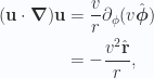
We found that after application of the perturbation

to the base state equations, our perturbed Navier-Stokes equation was

Application of the perturbation to the energy equation.

We’ve got

Using this, and 2.7, and neglecting any terms of second order smallness we have

We’d like to solve this and 2.13 simultaneously.
Non-dimensionalisation of the thermal velocity equation.
We’d like to scale
 latex d$} \\ t & \quad \mbox{with
  } \\ \delta w & \quad \mbox{with
  } \\ \delta T & \quad \mbox{with
  }\end{array}\end{aligned} \hspace{\stretch{1}}(3.17)$
Sanity check of dimensions
- viscosity dimensions
![\begin{aligned}[\nu] \sim \left[ \frac{1}{\text{T}} \right]/ \left[\frac{1}{{\text{L}^2}} \right] \sim \frac{\text{L}^2}{\text{T}},\end{aligned} \hspace{\stretch{1}}(3.18)](https://s0.wp.com/latex.php?latex=%5Cbegin%7Baligned%7D%5B%5Cnu%5D+%5Csim+%5Cleft%5B+%5Cfrac%7B1%7D%7B%5Ctext%7BT%7D%7D+%5Cright%5D%2F+%5Cleft%5B%5Cfrac%7B1%7D%7B%7B%5Ctext%7BL%7D%5E2%7D%7D+%5Cright%5D+%5Csim+%5Cfrac%7B%5Ctext%7BL%7D%5E2%7D%7B%5Ctext%7BT%7D%7D%2C%5Cend%7Baligned%7D+%5Chspace%7B%5Cstretch%7B1%7D%7D%283.18%29&bg=fafcff&fg=2a2a2a&s=0&c=20201002)
- thermal conductivity dimensionsSince
![[ \kappa \boldsymbol{\nabla}^2 ] \sim 1/\text{T}](https://s0.wp.com/latex.php?latex=%5B+%5Ckappa+%5Cboldsymbol%7B%5Cnabla%7D%5E2+%5D+%5Csim+1%2F%5Ctext%7BT%7D&bg=fafcff&fg=2a2a2a&s=0&c=20201002) , we have
, we have
![\begin{aligned}[ \kappa ] \sim \frac{\text{L}^2}{\text{T}}\end{aligned} \hspace{\stretch{1}}(3.19)](https://s0.wp.com/latex.php?latex=%5Cbegin%7Baligned%7D%5B+%5Ckappa+%5D+%5Csim+%5Cfrac%7B%5Ctext%7BL%7D%5E2%7D%7B%5Ctext%7BT%7D%7D%5Cend%7Baligned%7D+%5Chspace%7B%5Cstretch%7B1%7D%7D%283.19%29&bg=fafcff&fg=2a2a2a&s=0&c=20201002)
- time scaling
![\begin{aligned}\left[\frac{d^2}{\nu}\right] \sim \frac{\text{L}^2}{\text{L}^2 \text{T}^{-1}} \sim \text{T}.\end{aligned} \hspace{\stretch{1}}(3.20)](https://s0.wp.com/latex.php?latex=%5Cbegin%7Baligned%7D%5Cleft%5B%5Cfrac%7Bd%5E2%7D%7B%5Cnu%7D%5Cright%5D+%5Csim+%5Cfrac%7B%5Ctext%7BL%7D%5E2%7D%7B%5Ctext%7BL%7D%5E2+%5Ctext%7BT%7D%5E%7B-1%7D%7D+%5Csim+%5Ctext%7BT%7D.%5Cend%7Baligned%7D+%5Chspace%7B%5Cstretch%7B1%7D%7D%283.20%29&bg=fafcff&fg=2a2a2a&s=0&c=20201002)
- velocity scaling
![\begin{aligned}[\kappa/d] \sim \frac{\text{L}^2}{\text{T}} \frac{1}{{\text{L}}} \sim [\delta w]\end{aligned} \hspace{\stretch{1}}(3.21)](https://s0.wp.com/latex.php?latex=%5Cbegin%7Baligned%7D%5B%5Ckappa%2Fd%5D+%5Csim+%5Cfrac%7B%5Ctext%7BL%7D%5E2%7D%7B%5Ctext%7BT%7D%7D+%5Cfrac%7B1%7D%7B%7B%5Ctext%7BL%7D%7D%7D+%5Csim+%5B%5Cdelta+w%5D%5Cend%7Baligned%7D+%5Chspace%7B%5Cstretch%7B1%7D%7D%283.21%29&bg=fafcff&fg=2a2a2a&s=0&c=20201002)
Looks like everything checks out.
Let’s apply this rescaling to our perturbed velocity equation 2.13

Introducing the \textit{Rayleigh number}

and dropping primes, we have

My class notes original had  with the value

but performing this non-dimensionalization shows that this was either quoted incorrectly, or typed wrong in the heat of the moment. A check against the text shows (equation (9.27)), shows that 3.23 is correct.
Non-dimensionalization of the energy equation
Rescaling our energy equation 3.16 we find

Introducing the \textit{Prandtl number}

and dropping primes our non-dimensionalized energy equation takes the form

Normal mode analysis.
We’ve got a pair of nasty looking coupled equations 3.24, and 3.27. Repeated so that we can see them together
\begin{subequations}


\end{subequations}
it’s clear that we can decouple these by inserting 3.42 into 3.28a. Doing that gives us a beastly 6th order spatial equation for the perturbed temperature

It’s pointed out in the text we have all the  and
and  derivatives coming together we can apply separation of variables with

provided we introduce some restrictions on the form of  . Here
  (if real) is the growth rate. Applying the Laplacian to this assumed solution we find

where

For 3.31 to be separable we require a constant proportionality

or

Picking  so that we don’t have hyperbolic solutions,
  must have the form

where

Our separation of variables function now takes the form

Writing

our beastly equation to solve is then given by

This is now an equation for only 

Conceptually we have just a plain old LDE, and should we decide to expand this out we have something of the form

Our standard toolbox method to solve this is to assume a solution  and compute the characteristic equation. We’d have to solve

Let’s back up a bit instead. Looking back to 3.42, it’s clear that we’ll have the same separable form for our perturbed velocity since we have

where

Assuming a solution of the form

our velocity is then fully specified in terms of the temperature, since we have

Back to our coupled equations.
Having gleamed an idea what the form of our solutions is, we can simplify our original coupled system, writing
\begin{subequations}


\end{subequations}
Considering the boundary conditions, if the heating is even then at  we can’t have any variation with and , so can only have
  . Thus at the boundary, from 3.46a, we have

From the continuity equation  , the text argues that we also have
  on the boundary, so that on that plane we also have

Expanding out 3.47 then gives us

or

These boundary value constraints 3.48, and 3.50, plus the coupled system equations 3.46 are the complete problem to solve. To get a feel for the solution of this system, consider the system with the following simpler set of boundary value constraints

which in the text is described as the artificial problem of thermal instability for boundaries that are stress free (FIXME: it’s not clear to me what that means without some thought … return to this). For such a system on the boundaries  (noting that we are still in dimensionless quantities), we have solutions

Note that we have

Inserting 3.52 into our system 3.46, we have

For any  ,
,  , we must then have

For  , this gives us the critical value for the Rayleigh number

the value that separates our stable and unstable solutions. On the other hand for
 (
( ), we have an instable system.
 (), we have a stable system.
FIXME: The text has a positive sign on the  term above. He actually solves the quadratic for , but I don’t see how that would make a difference. Is there an error here, or a typo in the text?
This is illustrated in figure (2).

Critical Rayleigh's number.
The instability means that we’ll have instable flows as illustrated in figure (3)

Instability due to heating.
Solving for these critical points we find
\begin{subequations}


\end{subequations}
Multimedia presentations.
- Kelvin-Helmholtz instability.Colored salt water underneath, with unsalty water on top. Apparatus tilted causing flow of one over the other. Instability of the interface.
See [2] for a really cool animation of a simulation of this effect. It ends up looking very fractal. Also interesting is the picture of this observed for real in the atmosphere of Saturn.
- A simulated mushroom cloud occurring with one fluid seeping into another. This looks it matches what we find under Rayleigh-Taylor instability in [3].
- plume, motion up through a denser fluid.
- Plateau-Rayleigh instability. Drop pinching off. See instability in the fluid channel feeding the drop. A crude illustration of this can be found in figure (4).

Crude illustration of instability leading to a drop pinching off.
A better illustrations (and animations) can be found in [4].
- Jet of water injected into a rotating tub on a turntable. Jet forms and surfaces.
References
[1] D.J. Acheson. Elementary fluid dynamics. Oxford University Press, USA, 1990.
[2] Wikipedia. Kelvin-helmholtz instability — wikipedia, the free encyclopedia [online]. 2012. [Online; accessed 4-April-2012]. http://en.wikipedia.org/w/index.php?title=Kelvin\%E2\%80\%93Helmholtz_instability&oldid=484301421.
[3] Wikipedia. Rayleigh-taylor instability — wikipedia, the free encyclopedia [online]. 2012. [Online; accessed 4-April-2012]. http://en.wikipedia.org/w/index.php?title=Rayleigh\%E2\%80\%93Taylor_instability&oldid=483569989.
[4] Wikipedia. Plateau-rayleigh instability — wikipedia, the free encyclopedia [online]. 2012. [Online; accessed 4-April-2012]. http://en.wikipedia.org/w/index.php?title=Plateau\%E2\%80\%93Rayleigh_instability&oldid=478499841.


and
. You should find that these equations have relatively simple solutions, i.e.,
and
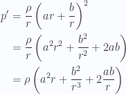
from the boundary conditions. Determine the pressure


 , and not
  ).
).
![\begin{aligned}(\hat{\mathbf{n}} \times (\boldsymbol{\nabla} \times \mathbf{u}) + 2 (\hat{\mathbf{n}} \cdot \boldsymbol{\nabla}) \mathbf{u})_i&=n_a (\boldsymbol{\nabla} \times \mathbf{u})_b \epsilon_{a b i} + 2 n_a \partial_a u_i \\ &=n_a \partial_r u_s \epsilon_{r s b} \epsilon_{a b i} + 2 n_a \partial_a u_i \\ &=n_a \partial_r u_s \delta_{ia}^{[rs]} + 2 n_a \partial_a u_i \\ &=n_a ( \partial_i u_a -\partial_a u_i ) + 2 n_a \partial_a u_i \\ &=n_a \partial_i u_a + n_a \partial_a u_i \\ &=n_a (\partial_i u_a + \partial_a u_i) \\ &=\sigma_{i a } n_a\end{aligned}](https://s0.wp.com/latex.php?latex=%5Cbegin%7Baligned%7D%28%5Chat%7B%5Cmathbf%7Bn%7D%7D+%5Ctimes+%28%5Cboldsymbol%7B%5Cnabla%7D+%5Ctimes+%5Cmathbf%7Bu%7D%29+%2B+2+%28%5Chat%7B%5Cmathbf%7Bn%7D%7D+%5Ccdot+%5Cboldsymbol%7B%5Cnabla%7D%29+%5Cmathbf%7Bu%7D%29_i%26%3Dn_a+%28%5Cboldsymbol%7B%5Cnabla%7D+%5Ctimes+%5Cmathbf%7Bu%7D%29_b+%5Cepsilon_%7Ba+b+i%7D++%2B+2+n_a+%5Cpartial_a+u_i+%5C%5C+%26%3Dn_a+%5Cpartial_r+u_s+%5Cepsilon_%7Br+s+b%7D+%5Cepsilon_%7Ba+b+i%7D++%2B+2+n_a+%5Cpartial_a+u_i+%5C%5C+%26%3Dn_a+%5Cpartial_r+u_s+%5Cdelta_%7Bia%7D%5E%7B%5Brs%5D%7D+%2B+2+n_a+%5Cpartial_a+u_i+%5C%5C+%26%3Dn_a+%28+%5Cpartial_i+u_a+-%5Cpartial_a+u_i+%29+%2B+2+n_a+%5Cpartial_a+u_i+%5C%5C+%26%3Dn_a+%5Cpartial_i+u_a+%2B+n_a+%5Cpartial_a+u_i+%5C%5C+%26%3Dn_a+%28%5Cpartial_i+u_a+%2B+%5Cpartial_a+u_i%29+%5C%5C+%26%3D%5Csigma_%7Bi+a+%7D+n_a%5Cend%7Baligned%7D+&bg=fafcff&fg=2a2a2a&s=0&c=20201002)


 and
and  , we have only one cross term and our curl is
 .
.


 .
.


 .
. normal direction will not have any cross terms


 .
. direction. The directional derivative portion of our strain will be a bit more work to compute because we have
  variation of the unit vectors


 is a constant in


 (a constant, which will also kill the
  term in the N-S equation). This isn’t really justified by anything we’ve done so far, but asking about this in class, it was stated that this is a restriction for this formulation of the Blasius problem.
![[\sqrt{\nu x/U}] = \sqrt{ (L^2/T) (L) (T/L)} = L](https://s0.wp.com/latex.php?latex=%5B%5Csqrt%7B%5Cnu+x%2FU%7D%5D+%3D+%5Csqrt%7B+%28L%5E2%2FT%29+%28L%29+%28T%2FL%29%7D+%3D+L&bg=fafcff&fg=2a2a2a&s=0&c=20201002) , but where did this definition of
, but where did this definition of  come from?


 latex \eta = 0$} \\ f’ = 1 & \quad \mbox{
 } \\ \end{array}\end{aligned} \hspace{\stretch{1}}(3.25)$

 is to be determined, and is scaled by our characteristic velocity
  . Observe that, as above, we are assuming that
  , a constant (which also kills off the
  term in the Navier-Stokes equation.) Given this form of
  , we note that

 to be a streamline, so that
  implying that
  . I don’t honestly follow the rational for that, but it’s certainly convenient to set
 is necessarily zero with this definition. We can now write
 we also have a function of
  to start with
 , but
, but  , so we’ve now got both
  and their derivatives


 )
)
 (to make this equation as easy to solve as possible), we can integrate to find the required form of
  . This gives

 , so we should set
  . This leaves us with


 and 3.37d, and 3.38c follows from the fact that


 .
.


 , we can write
 we have
 and
and  . The exact solution of this ill conditioned differential equation is

 we have approximately
 ,
,  we have approximately
 . For
. For  a constant pressure gradient
  is imposed. Show that
  satifies
 .
.


 , allows for solutions
 ).
). .
.
 , our equation takes the form


 constant into the equation as an integration constant has been employed, knowing that it will kill the
  contributions at
 , and subtracting gives us
  , so a specific solution that matches our required boundary value (and initial value) conditions is just the steady state channel flow solution we are familiar with


 , yielding

 has been used assuming that we want a solution that is damped with time.

 due to our boundary value conditions. For our sin terms to be solutions we require


 latex m$ even} \\ \cos \left( \frac{ m \pi y }{2 h} \right) & \quad \mbox{
 odd} \\ \end{array}\right.\end{aligned} \hspace{\stretch{1}}(2.26)$
 2.16b, leaving us to solve the Fourier problem
 latex m$ even} \\ \cos \left( \frac{ m \pi y }{2 h} \right) & \quad \mbox{
 term
term
 must be odd,
  for some integer
  , so this integral is zero unless
  (consider
  ). For the

 , we have

 term which is
 these terms all die off, leaving us with just the steady state.
 , and
, and  (parameterizing the pressure gradient by the average velocity it will induce), a plot of the parabola that we are fitting to and the difference of that from the first Fourier term is shown in figure (1).
 of the height of the parabola. This is illustrated in figure (2) where the magnitude of the first 5 deviations from the steady state are plotted.

 , and
, and  we’ll look at the second order ill conditioned LDE


 , then we have

 then we have to be more careful constructing an approximation. When
  is also of the same order of smallness we have


 . This gives us


 and
and  to be determined from our boundary value conditions. We find
 and by subtracting


 we have


 we have


 is the coefficient of volume expansion,
  length scale associated with the problem,
  is the applied temperature difference,
  is the kinematic viscosity and
  is the thermal diffusivity.
  :
:
![\begin{aligned}\left[ \frac{\partial {\mathbf{u}}}{\partial {t}} \right] = [ \nu \boldsymbol{\nabla}^2 \mathbf{u} ]\end{aligned} \hspace{\stretch{1}}(2.1)](https://s0.wp.com/latex.php?latex=%5Cbegin%7Baligned%7D%5Cleft%5B+%5Cfrac%7B%5Cpartial+%7B%5Cmathbf%7Bu%7D%7D%7D%7B%5Cpartial+%7Bt%7D%7D+%5Cright%5D+%3D+%5B+%5Cnu+%5Cboldsymbol%7B%5Cnabla%7D%5E2+%5Cmathbf%7Bu%7D+%5D%5Cend%7Baligned%7D+%5Chspace%7B%5Cstretch%7B1%7D%7D%282.1%29&bg=fafcff&fg=2a2a2a&s=0&c=20201002)
![\begin{aligned}[\nu] = \frac{1}{{[t] [\boldsymbol{\nabla}^2]}} = \frac{1}{{T}} L^2\end{aligned} \hspace{\stretch{1}}(2.2)](https://s0.wp.com/latex.php?latex=%5Cbegin%7Baligned%7D%5B%5Cnu%5D+%3D+%5Cfrac%7B1%7D%7B%7B%5Bt%5D+%5B%5Cboldsymbol%7B%5Cnabla%7D%5E2%5D%7D%7D+%3D+%5Cfrac%7B1%7D%7B%7BT%7D%7D+L%5E2%5Cend%7Baligned%7D+%5Chspace%7B%5Cstretch%7B1%7D%7D%282.2%29&bg=fafcff&fg=2a2a2a&s=0&c=20201002)
![\begin{aligned}[\alpha] = \frac{1}{{[V]}} \left[ \frac{\partial {V}}{\partial {T}} \right] = \frac{1}{{[K]}},\end{aligned} \hspace{\stretch{1}}(2.3)](https://s0.wp.com/latex.php?latex=%5Cbegin%7Baligned%7D%5B%5Calpha%5D+%3D+%5Cfrac%7B1%7D%7B%7B%5BV%5D%7D%7D+%5Cleft%5B+%5Cfrac%7B%5Cpartial+%7BV%7D%7D%7B%5Cpartial+%7BT%7D%7D+%5Cright%5D+%3D+%5Cfrac%7B1%7D%7B%7B%5BK%5D%7D%7D%2C%5Cend%7Baligned%7D+%5Chspace%7B%5Cstretch%7B1%7D%7D%282.3%29&bg=fafcff&fg=2a2a2a&s=0&c=20201002)
![\begin{aligned}[U_1] = \frac{L}{T \not{{T}}} \not{{\frac{1}{{K}}}} L^2 \not{{K}} \frac{\not{{T}}}{L^2} = \frac{L}{T}\end{aligned} \hspace{\stretch{1}}(2.4)](https://s0.wp.com/latex.php?latex=%5Cbegin%7Baligned%7D%5BU_1%5D+%3D+%5Cfrac%7BL%7D%7BT+%5Cnot%7B%7BT%7D%7D%7D+%5Cnot%7B%7B%5Cfrac%7B1%7D%7B%7BK%7D%7D%7D%7D+L%5E2+%5Cnot%7B%7BK%7D%7D+%5Cfrac%7B%5Cnot%7B%7BT%7D%7D%7D%7BL%5E2%7D+%3D+%5Cfrac%7BL%7D%7BT%7D%5Cend%7Baligned%7D+%5Chspace%7B%5Cstretch%7B1%7D%7D%282.4%29&bg=fafcff&fg=2a2a2a&s=0&c=20201002)
 :
:
![\begin{aligned}[U_2] = \frac{L^2}{T} \frac{1}{{L}} = \frac{L}{T}.\end{aligned} \hspace{\stretch{1}}(2.5)](https://s0.wp.com/latex.php?latex=%5Cbegin%7Baligned%7D%5BU_2%5D+%3D+%5Cfrac%7BL%5E2%7D%7BT%7D+%5Cfrac%7B1%7D%7B%7BL%7D%7D+%3D+%5Cfrac%7BL%7D%7BT%7D.%5Cend%7Baligned%7D+%5Chspace%7B%5Cstretch%7B1%7D%7D%282.5%29&bg=fafcff&fg=2a2a2a&s=0&c=20201002)

![\begin{aligned}[U_3] = \sqrt{ \frac{L}{T^2} \frac{1}{{K}} L K } = \frac{L}{T}\end{aligned} \hspace{\stretch{1}}(2.6)](https://s0.wp.com/latex.php?latex=%5Cbegin%7Baligned%7D%5BU_3%5D+%3D+%5Csqrt%7B+%5Cfrac%7BL%7D%7BT%5E2%7D+%5Cfrac%7B1%7D%7B%7BK%7D%7D+L+K+%7D+%3D+%5Cfrac%7BL%7D%7BT%7D%5Cend%7Baligned%7D+%5Chspace%7B%5Cstretch%7B1%7D%7D%282.6%29&bg=fafcff&fg=2a2a2a&s=0&c=20201002)


![\begin{aligned}[\kappa] = \frac{1}{{[t][\boldsymbol{\nabla}^2]}} = \frac{L^2}{T}\end{aligned} \hspace{\stretch{1}}(2.8)](https://s0.wp.com/latex.php?latex=%5Cbegin%7Baligned%7D%5B%5Ckappa%5D+%3D+%5Cfrac%7B1%7D%7B%7B%5Bt%5D%5B%5Cboldsymbol%7B%5Cnabla%7D%5E2%5D%7D%7D+%3D+%5Cfrac%7BL%5E2%7D%7BT%7D%5Cend%7Baligned%7D+%5Chspace%7B%5Cstretch%7B1%7D%7D%282.8%29&bg=fafcff&fg=2a2a2a&s=0&c=20201002)
![\begin{aligned}[U_4] = \frac{L^2}{T} \frac{1}{{L}} = \frac{L}{T}.\end{aligned} \hspace{\stretch{1}}(2.9)](https://s0.wp.com/latex.php?latex=%5Cbegin%7Baligned%7D%5BU_4%5D+%3D+%5Cfrac%7BL%5E2%7D%7BT%7D+%5Cfrac%7B1%7D%7B%7BL%7D%7D+%3D+%5Cfrac%7BL%7D%7BT%7D.%5Cend%7Baligned%7D+%5Chspace%7B%5Cstretch%7B1%7D%7D%282.9%29&bg=fafcff&fg=2a2a2a&s=0&c=20201002)

 layer depth and a ten degree temperature drop convective velocities have been experimentally measured of about
  .
. , calculate the values of
  ,
,  do you think are suitable for nondimensionalising the velocity in Navier-Stokes/Energy equation describing the water convection problem?

 . Which of the characteristic velocities should we use to nondimensionalise Navier-Stokes/Energy equations describing mantle convection?

 , where
  is the characteristic length scale,
 ,
,
 and Froude number
  .
. , to make all terms (most obviously the


 replacement, using the Froude number, we have
 we tidy things up a bit, and also allow for insertion of the Reynold’s number
![\begin{aligned}[\text{Fr}] = [g] T = \frac{L}{T},\end{aligned} \hspace{\stretch{1}}(3.27)](https://s0.wp.com/latex.php?latex=%5Cbegin%7Baligned%7D%5B%5Ctext%7BFr%7D%5D+%3D+%5Bg%5D+T+%3D+%5Cfrac%7BL%7D%7BT%7D%2C%5Cend%7Baligned%7D+%5Chspace%7B%5Cstretch%7B1%7D%7D%283.27%29&bg=fafcff&fg=2a2a2a&s=0&c=20201002)
 . What is the phase difference between the velocity of the plate
  and the shear stress on the plate?


 . The shear stress at the plate lags the driving velocity by 90 degrees.


 changes with time after making it. In a stable configuration without friction we will induce an oscillation as plotted in figure (\ref{fig:continuumL21:continuumL21Fig2a}) for the parabolic configuration. With friction we’ll have a damping effect. This is plotted for the parabolic well in figure (\ref{fig:continuumL21:continuumL21Fig2b}).


 but still
  , but these are less common.


 initially (our base state), we’ll call the following the equation of the base state


 we have

 is constant (actually that’s already been done above), we can cancel it, leaving
 we have


 are
are

 , this should look something like figure (\ref{fig:continuumProblemSet2:continuumProblemSet2Fig4}) whereas for the higher viscosity on the top, these would be roughly flipped as in figure (\ref{fig:continuumProblemSet2:continuumProblemSet2Fig5}).

 term in the Navier-Stokes equations for these systems.
 and
and  respectively, and let the heights from the interface be
  and
and  respectively.
 and
and  (the lower and upper walls respectively). Clearly the integration constants
  are just the velocities. Matching the tangential component of the traction vectors at


 ,
,  , showing the superposition of the shear and channel flow solutions can be found here
 , this is plotted