Peeter Joot's (OLD) Blog.

Math, physics, perl, and programming obscurity.

Posts Tagged ‘torque’

Couette flow of a viscous incompressible fluid (visualizing it).

Posted by peeterjoot on April 12, 2012

[Click here for a PDF of this post(and previous).]

In Couette flow of a viscous incompressible fluid, I looked at solving this problem. As a followup, here are some visualizations of the velocity field as the outer cylinder angular velocity is changed.

The Mathematica workbook that was used to generate the figures is also available for more direct play, and includes slider controls for the cylinder radii and angular velocities.

Posted in Math and Physics Learning. | Tagged: , , , , , , | Leave a Comment »

Couette flow of a viscous incompressible fluid.

Posted by peeterjoot on April 9, 2012

[Click here for a PDF of this post with nicer formatting (especially if my latex to wordpress script has left FORMULA DOES NOT PARSE errors.)]

Motivation.

A problem from this years phy1530 problem set 2 that appears appropriate for phy454 exam prep.

Statement.

Consider the steady flow between two long cylinders of radii R_1 and R_2, R_1 > R_1, rotating about their axes with angular velocities \Omega_1, \Omega_2. Look for a solution of the form, where \hat{\boldsymbol{\phi}} is a unit vector along the azimuthal direction:

\begin{subequations}

\begin{aligned}\mathbf{u} = v(r) \hat{\boldsymbol{\phi}}\end{aligned} \hspace{\stretch{1}}(2.1a)

\begin{aligned}p = p(r).\end{aligned} \hspace{\stretch{1}}(2.1b)

\end{subequations}

  • Write out the Navier-Stokes equations and find differential equations for v(r) and p(r). You should find that these equations have relatively simple solutions, i.e.,

    \begin{aligned}v(r) = a r + \frac{b}{r}.\end{aligned} \hspace{\stretch{1}}(2.2)

  • Fix gthe constants a and b from the boundary conditions. Determine the pressure p(r).
  • Compute the friction forces that the fluid exerts on the cylinders, and compute the torque on each cylinder. Show that the total torque on the fluid is zero (as must be the case).

This is also a problem that I recall was outlined in section 2 from [1]. Some of the instabilities that are mentioned in the text are nicely illustrated in [2].

We illustrate our system in figure (1).

Figure 1: Coutette flow configuration


Solution: Part 1. Navier-Stokes and resulting differential equations.

Navier-Stokes for steady state incompressible flow has the form

\begin{subequations}

\begin{aligned}(\mathbf{u} \cdot \boldsymbol{\nabla}) \mathbf{u} = -\frac{1}{{\rho}} \boldsymbol{\nabla} p + \nu \boldsymbol{\nabla}^2 \mathbf{u}\end{aligned} \hspace{\stretch{1}}(3.3a)

\begin{aligned}\boldsymbol{\nabla} \cdot \mathbf{u} = 0.\end{aligned} \hspace{\stretch{1}}(3.3b)

\end{subequations}

where the gradient has the form

\begin{aligned}\boldsymbol{\nabla} = \hat{\mathbf{r}} \partial_r + \frac{\hat{\boldsymbol{\phi}}}{r} \partial_\phi.\end{aligned} \hspace{\stretch{1}}(3.4)

Let’s first verify that the incompressible condition 3.3b is satisfied for the presumed form of the solution we seek. We have

\begin{aligned}\boldsymbol{\nabla} \cdot \mathbf{u} &=\left( \hat{\mathbf{r}} \partial_r + \frac{\hat{\boldsymbol{\phi}}}{r} \partial_\phi \right) \cdot (v(r) \hat{\boldsymbol{\phi}}(\phi) ) \\ &=(\hat{\mathbf{r}} \cdot \hat{\boldsymbol{\phi}}) v' + \frac{\hat{\boldsymbol{\phi}}^2}{r} \partial_\phi v(r)+ \frac{v(r) \hat{\boldsymbol{\phi}}}{r} \cdot \partial_\phi \hat{\boldsymbol{\phi}} \\ &= \frac{v(r) \hat{\boldsymbol{\phi}}}{r} \cdot (-\hat{\mathbf{r}}) \\ &= 0\end{aligned}

Good. Now let’s write out the terms of the momentum conservation equation 3.3a. We’ve got
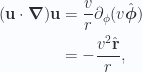
\begin{aligned}(\mathbf{u} \cdot \boldsymbol{\nabla}) \mathbf{u}&=\frac{ v}{r} \partial_\phi ( v \hat{\boldsymbol{\phi}} ) \\ &=-\frac{ v^2 \hat{\mathbf{r}}}{r},\end{aligned}

and

\begin{aligned}-\frac{1}{{\rho}} \boldsymbol{\nabla} p&=-\frac{1}{{\rho}} \left( \hat{\mathbf{r}} \partial_r + \frac{\hat{\boldsymbol{\phi}}}{r} \partial_\phi \right) p(r) \\ &=-\frac{\hat{\mathbf{r}} p'}{\rho},\end{aligned}

and

\begin{aligned}\nu \boldsymbol{\nabla}^2 \mathbf{u}&=\nu \left( \hat{\mathbf{r}} \partial_r + \frac{\hat{\boldsymbol{\phi}}}{r} \partial_\phi \right) \cdot\left( \hat{\mathbf{r}} \partial_r + \frac{\hat{\boldsymbol{\phi}}}{r} \partial_\phi \right) (v(r) \hat{\boldsymbol{\phi}}(\phi)) \\ &=\nu \left( \partial_{rr} + \frac{1}{{r^2}} \partial_{\phi\phi}+ \frac{\hat{\boldsymbol{\phi}}}{r} \partial_\phi \cdot (\hat{\mathbf{r}} \partial_r)\right)(v(r) \hat{\boldsymbol{\phi}}(\phi)) \\ &=\nu \left( \partial_{rr} + \frac{1}{{r^2}} \partial_{\phi\phi}+ \frac{1}{r} \partial_r\right)(v(r) \hat{\boldsymbol{\phi}}(\phi)) \\ &=\nu \left( \frac{1}{{r}} \partial_{r} (r \partial_r) + \frac{1}{{r^2}} \partial_{\phi\phi}\right)(v(r) \hat{\boldsymbol{\phi}}(\phi)) \\ &=\nu \left( \frac{1}{{r}} (r v')' - \frac{v}{r^2} \right)\hat{\boldsymbol{\phi}}\end{aligned}

Equating \hat{\mathbf{r}} and \hat{\boldsymbol{\phi}} components we have two equations to solve

\begin{subequations}

\begin{aligned}r (r v')' - v = 0\end{aligned} \hspace{\stretch{1}}(3.5a)

\begin{aligned}p' = \frac{\rho v^2}{r}.\end{aligned} \hspace{\stretch{1}}(3.5b)

\end{subequations}

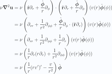
Expanding out our velocity equation we have

\begin{aligned}r^2 v'' + r v' - v = 0,\end{aligned} \hspace{\stretch{1}}(3.6)

for which we’ve been told to expect that 2.2 is a solution (and it has the two integration constants we require for a solution to a homogeneous equation of this form). Let’s verify that we’ve computed the correct differential equation for the problem by trying this solution

\begin{aligned}r^2 v'' + r v' - v &=r^2 \left( a -\frac{b}{r^2} \right)' + r \left( a -\frac{b}{r^2} \right) - a r - \frac{b}{r} \\ &=r^2 \frac{2 b}{r^3} + \not{{a r}} - \frac{b}{r} - \not{{a r}} - \frac{b}{r} \\ &=\frac{2 b}{r} - \frac{2 b}{r} \\ &= 0.\end{aligned}

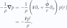
Given the velocity, we can now determine the pressure up to a constant
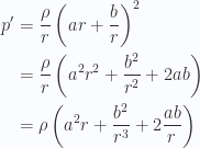
\begin{aligned}p' &= \frac{\rho}{r} \left( a r + \frac{b}{r} \right)^2 \\ &= \frac{\rho}{r} \left( a^2 r^2 + \frac{b^2}{r^2} + 2 a b \right) \\ &= \rho \left( a^2 r + \frac{b^2}{r^3} + 2 \frac{a b}{r} \right)\end{aligned}

so

\begin{aligned}p_r -p_0= \rho \left( \frac{1}{{2}} a^2 r^2 - \frac{b^2}{2 r^2} + 2 a b \ln r \right)\end{aligned} \hspace{\stretch{1}}(3.7)

Solution: Part 2. Fixing the constants.

To determine our integration constants we recall that velocity associated with a radial position \mathbf{x} = r \hat{\mathbf{r}} in cylindrical coordinates takes the form

\begin{aligned}\frac{\mathbf{x}}{dt} = \dot{r} \hat{\mathbf{r}} + r \hat{\boldsymbol{\phi}} \dot{\phi},\end{aligned} \hspace{\stretch{1}}(4.8)

where \dot{\phi} is the angular velocity. The cylinder walls therefore have the velocity

\begin{aligned}v = r \dot{\phi},\end{aligned} \hspace{\stretch{1}}(4.9)

so our boundary conditions (given a no-slip assumption for the fluids) are

\begin{aligned}v(R_1) &= R_1 \Omega_1 \\ v(R_2) &= R_2 \Omega_2.\end{aligned} \hspace{\stretch{1}}(4.10)

This gives us a pair of equations to solve for a and b

\begin{aligned}R_1 \Omega_1 &= a R_1 + \frac{b}{R_1} \\ R_2 \Omega_2 &= a R_2 + \frac{b}{R_2}.\end{aligned} \hspace{\stretch{1}}(4.12)

Multipling each by R_1 and R_2 respectively gives us

\begin{aligned}b = R_1^2 (\Omega_1 - a) = R_2^2 (\Omega_2 - a).\end{aligned} \hspace{\stretch{1}}(4.14)

Rearranging for a we find

\begin{aligned}R_1^2 \Omega_1 - R_2^2 \Omega_2 = (R_1^2 - R_2^2) a,\end{aligned} \hspace{\stretch{1}}(4.15)

or

\begin{aligned}a = \frac{ R_2^2 \Omega_2 - R_1^2 \Omega_1}{R_2^2 - R_1^2}.\end{aligned} \hspace{\stretch{1}}(4.16)

For b we have

\begin{aligned}b &= R_1^2 (\Omega_1 - a) \\ &=\frac{R_1^2 }{R_2^2 - R_1^2}(\Omega_1 ( R_2^2 - \not{{R_1^2}}) - R_2^2 \Omega_2 + \not{{R_1^2 \Omega_1}}),\end{aligned}

or

\begin{aligned}b = \frac{R_1^2 R_2^2}{R_2^2 - R_1^2} (\Omega_1 -\Omega_2).\end{aligned} \hspace{\stretch{1}}(4.17)

This gives us

\begin{subequations}

\begin{aligned}v(r) = \frac{1}{{R_2^2 - R_1^2}}\left(\left( R_2^2 \Omega_2 - R_1^2 \Omega_1\right) r+\frac{R_1^2 R_2^2}{r} (\Omega_1 -\Omega_2)\right)\end{aligned} \hspace{\stretch{1}}(4.18a)

\begin{aligned}\begin{aligned}p_r -&p_0= \frac{\rho }{(R_2^2 - R_1^2)^2} \times \\ &\left( \frac{1}{{2}} \left( R_2^2 \Omega_2 - R_1^2 \Omega_1\right)^2r^2 -\frac{R_1^4 R_2^4}{2 r^2} (\Omega_1 - \Omega_2)^2+ 2 \left( R_2^2 \Omega_2 - R_1^2 \Omega_1\right) R_1^4 R_2^4 (\Omega_1 - \Omega_2)^2 \ln r\right).\end{aligned}\end{aligned} \hspace{\stretch{1}}(4.18b)

\end{subequations}

Solution: Part 3. Friction and torque.

We can expand out the identity for the traction vector

\begin{aligned}\mathbf{t} = \mathbf{e}_i \sigma_{ij} n_j= -p \hat{\mathbf{n}} + \mu \left( 2 (\hat{\mathbf{n}} \cdot \boldsymbol{\nabla}) \mathbf{u} + \hat{\mathbf{n}} \times (\boldsymbol{\nabla} \times \mathbf{u})\right),\end{aligned} \hspace{\stretch{1}}(5.19)

in cylindrical coordinates and find

\begin{subequations}

\begin{aligned}\sigma_{rr}=-p + 2 \mu \not{{\frac{\partial {u_r}}{\partial {r}}}}\end{aligned} \hspace{\stretch{1}}(5.20a)

\begin{aligned}\sigma_{\phi \phi}=-p + 2 \mu \left(\frac{1}{{r}}\not{{\frac{\partial {u_\phi}}{\partial {\phi}}}} + \not{{\frac{u_r}{r}}}\right)\end{aligned} \hspace{\stretch{1}}(5.20b)

\begin{aligned}\sigma_{z z}=-p + 2 \mu \not{{\frac{\partial {u_z}}{\partial {z}}}}\end{aligned} \hspace{\stretch{1}}(5.20c)

\begin{aligned}\sigma_{r \phi}=\mu \left( \frac{\partial {u_\phi}}{\partial {r}}+\frac{1}{{r}} \not{{\frac{\partial {u_r}}{\partial {\phi}}}}- \frac{u_\phi}{r}\right)\end{aligned} \hspace{\stretch{1}}(5.20d)

\begin{aligned}\sigma_{\phi z}=\mu \left(\frac{1}{r} \not{{\frac{\partial {u_z}}{\partial {\phi}}}} + \not{{\frac{\partial {u_\phi}}{\partial {z}}}}\right)\end{aligned} \hspace{\stretch{1}}(5.20e)

\begin{aligned}\sigma_{z r}=\mu \left(\not{{\frac{\partial {u_r}}{\partial {z}}}}+ \not{{\frac{\partial {u_z}}{\partial {r}}}}\right),\end{aligned} \hspace{\stretch{1}}(5.20f)

\end{subequations}

so we have

\begin{subequations}

\begin{aligned}\sigma_{rr} = \sigma_{\phi \phi} = \sigma_{z z} = -p \end{aligned} \hspace{\stretch{1}}(5.21a)

\begin{aligned}\sigma_{\phi z} = \sigma_{z r} = 0\end{aligned} \hspace{\stretch{1}}(5.21b)

\begin{aligned}\sigma_{r \phi} = \mu \left( \frac{\partial {u_\phi}}{\partial {r}} - \frac{u_\phi}{r} \right)\end{aligned} \hspace{\stretch{1}}(5.21c)

\end{subequations}

We want to expand the last of these

\begin{aligned}\sigma_{r \phi} &= \mu \left( \frac{\partial {u_\phi}}{\partial {r}} - \frac{u_\phi}{r} \right) \\ &= \mu \left( a r + \frac{b}{r}\right)' \\ &= \mu \left( a - \frac{b}{r^2}\right).\end{aligned}

So the traction vector, our force per unit area on the fluid at the inner surface (where the normal is \hat{\mathbf{r}}), is

\begin{aligned}\mathbf{t}_1 = -p \hat{\mathbf{r}} + \mu \left( a - \frac{b}{r^2} \right) \hat{\boldsymbol{\phi}},\end{aligned} \hspace{\stretch{1}}(5.22)

and our torque per unit area from the inner cylinder on the fluid is thus

\begin{aligned}\boldsymbol{\tau}_1 = r \hat{\mathbf{r}} \times \mathbf{t} = r \mu \left( a - \frac{b}{r^2} \right) \hat{\mathbf{z}}.\end{aligned} \hspace{\stretch{1}}(5.23)

Observing that our stress tensors flip sign for an inwards normal, our torque per unit area from the outer cylinder is

\begin{aligned}\boldsymbol{\tau}_2 = r \hat{\mathbf{r}} \times (-\mathbf{t}_1) = -r \mu \left( a - \frac{b}{r^2} \right) \hat{\mathbf{z}}.\end{aligned} \hspace{\stretch{1}}(5.24)

For the complete torque on the fluid due to a strip of width \Delta z the magnitudes of the total torque from each cylinder are respectively

\begin{aligned}\tau_1 = 2 \pi r^2 \Delta z \mu \left( a - \frac{b}{r^2} \right)\end{aligned} \hspace{\stretch{1}}(5.25)

\begin{aligned}\tau_2 = - 2 \pi r^2 \Delta z \mu \left( a - \frac{b}{r^2} \right)\end{aligned} \hspace{\stretch{1}}(5.26)

As expected these torques on the fluids sum to zero

\begin{aligned}\tau_2 + \tau_1 = 0.\end{aligned} \hspace{\stretch{1}}(5.27)

Evaluating these at R_1 and R_2 respectively gives us the torques on the fluid by the cylinders, so inverting these provides the torques on the cylinders by the fluid

\begin{aligned}\text{torque on inner cylinder (1) by the fluid} = -(2 \pi R_1^2) \Delta z \mu \left( a - \frac{b}{R_1^2} \right).\end{aligned} \hspace{\stretch{1}}(5.28)

For the outer cylinder the total torque on a strip of width \Delta z is

\begin{aligned}\text{torque on outer cylinder (2) by the fluid} = (2 \pi R_2^2) \Delta z \mu \left( a - \frac{b}{R_2^2} \right).\end{aligned} \hspace{\stretch{1}}(5.29)

References

[1] D.J. Acheson. Elementary fluid dynamics. Oxford University Press, USA, 1990.

[2] Wikipedia. Taylor-couette flow — wikipedia, the free encyclopedia [online]. 2012. [Online; accessed 10-April-2012]. http://en.wikipedia.org/w/index.php?title=Taylor\%E2\%80\%93Couette_flow&oldid=483281707.

Posted in Math and Physics Learning. | Tagged: , , , , , | Leave a Comment »