Disclaimer.
Peeter’s lecture notes from class. May not be entirely coherent.
Rotation operator in spin space.
We can formally expand our rotation operator in Taylor series

or

where we’ve used the fact that 
So our representation of the spin operator is

Note that, in particular,

This “rotates” the ket, but introduces a phase factor.
Can do this in general for other degrees of spin, for 
Unfortunate interjection by me
I mentioned the half angle rotation operator that requires a half angle operator sandwich. Prof. Sipe thought I might be talking about a Heisenberg picture representation, where we have something like this in expectation values

so that

However, what I was referring to, was that a general rotation of a vector in a Pauli matrix basis

can be expressed by sandwiching the Pauli vector representation by two half angle rotation operators like our spin 1/2 operators from class today

where 

For example, rotating in the 


Observe that these exponentials commute with 

yielding our usual coordinate rotation matrix. Expressed in terms of a unit normal to that plane, we form the normal by multiplication with the unit spatial volume element 

and can in general write a spatial rotation in a Pauli basis representation as a sandwich of half angle rotation matrix exponentials

when 


I believe it was pointed out in one of [1] or [2] that rotations expressed in terms of half angle Pauli matrices has caused some confusion to students of quantum mechanics, because this 
The book [1] takes this a lot further, and produces a formulation of spin operators that is devoid of the normal scalar imaginary 
Spin dynamics
At least classically, the angular momentum of charged objects is associated with a magnetic moment as illustrated in figure (\ref{fig:qmTwoL15:qmTwoL15fig1})
\begin{figure}[htp]
\centering
\includegraphics[totalheight=0.2\textheight]{qmTwoL15fig1}
\caption{Magnetic moment due to steady state current}
\end{figure}

In our scheme, following the (cgs?) text conventions of [3], where the 


For a charge moving in a circle as in figure (\ref{fig:qmTwoL15:qmTwoL15fig2})
\begin{figure}[htp]
\centering
\includegraphics[totalheight=0.2\textheight]{qmTwoL15fig2}
\caption{Charge moving in circle.}
\end{figure}
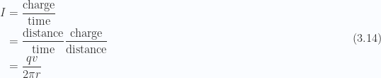
so the magnetic moment is

Here 
Recall that we have a torque, as shown in figure (\ref{fig:qmTwoL15:qmTwoL15fig3})
\begin{figure}[htp]
\centering
\includegraphics[totalheight=0.2\textheight]{qmTwoL15fig3}
\caption{Induced torque in the presence of a magnetic field.}
\end{figure}

tending to line up 

Also recall that this torque leads to precession as shown in figure (\ref{fig:qmTwoL15:qmTwoL15fig4})

\begin{figure}[htp]
\centering
\includegraphics[totalheight=0.2\textheight]{qmTwoL15fig4}
\caption{Precession due to torque.}
\end{figure}
with precession frequency

For a current due to a moving electron

where we are, here, writing for charge on the electron 
Question: steady state currents only?. Yes, this is only true for steady state currents.
For the translational motion of an electron, even if it is not moving in a steady way, regardless of it’s dynamics

Now, back to quantum mechanics, we turn 


What about the “spin”?
Perhaps

we write this as

so that

Experimentally, one finds to very good approximation

There was a lot of trouble with this in early quantum mechanics where people got things wrong, and canceled the wrong factors of 
In fact, Dirac’s relativistic theory for the electron predicts 
When this is measured experimentally, one does not get exactly

Richard Feynman compared the precision of quantum mechanics, referring to this measurement, “to predicting a distance as great as the width of North America to an accuracy of one human hair’s breadth”.
References
[1] C. Doran and A.N. Lasenby. Geometric algebra for physicists. Cambridge University Press New York, Cambridge, UK, 1st edition, 2003.
[2] D. Hestenes. New Foundations for Classical Mechanics. Kluwer Academic Publishers, 1999.
[3] BR Desai. Quantum mechanics with basic field theory. Cambridge University Press, 2009.
 latex x \in [0,a]$} \\ \infty & \quad \mbox{otherwise} \\ \end{array}\right.\end{aligned} \hspace{\stretch{1}}(2.1)$


 , we have


 .
.


 is the electric field.

 , and
, and  we have a 4 fold degeneracy


 leaving


 into this we have, for


 perturbation of
  we can from 4.36 write the exact generalization of 4.32 as
 and take a slightly different approach. We can find Prof Sipe’s final result with a bit less work, if a hybrid of the two methods is used.


 instead of the
  that we used in class because its easier to write.


 (using the notation in the text, not in class) is to be determined.
 come from in our superposition state? We will see after we start taking derivatives that this is what we need to cancel the
  in Schr\”{o}dinger’s equation.


 coefficients, and we can refer to the class notes for that without change.


 , let’s call it

 is implied.
 as
as
 which acts on
  , which is now an operator that acts on


 commute)


 is an eigenket of
  with eigenvalue
  .
.
 .
. ?
? projected down onto the
  plane at angle
  and at an angle
  from the
  axis.
axis. since there is nothing special about the


![\begin{aligned}\left[{\sigma_i},{\sigma_j}\right] = \sigma_i \sigma_j + \sigma_j \sigma_i = 0, \qquad \mbox{ if](https://s0.wp.com/latex.php?latex=%5Cbegin%7Baligned%7D%5Cleft%5B%7B%5Csigma_i%7D%2C%7B%5Csigma_j%7D%5Cright%5D+%3D+%5Csigma_i+%5Csigma_j+%2B+%5Csigma_j+%5Csigma_i+%3D+0%2C+%5Cqquad+%5Cmbox%7B+if+&bg=fafcff&fg=2a2a2a&s=0&c=20201002) latex i < j$}\end{aligned} \hspace{\stretch{1}}(4.46)$
latex i < j$}\end{aligned} \hspace{\stretch{1}}(4.46)$


 )
)![\begin{aligned}\left[{\sigma_i},{\sigma_j}\right] &= 2 \delta_{ij} \sigma_0 \\ \left[{\sigma_x},{\sigma_y}\right] &= 2 i \sigma_z\end{aligned} \hspace{\stretch{1}}(4.52)](https://s0.wp.com/latex.php?latex=%5Cbegin%7Baligned%7D%5Cleft%5B%7B%5Csigma_i%7D%2C%7B%5Csigma_j%7D%5Cright%5D+%26%3D+2+%5Cdelta_%7Bij%7D+%5Csigma_0+%5C%5C+%5Cleft%5B%7B%5Csigma_x%7D%2C%7B%5Csigma_y%7D%5Cright%5D+%26%3D+2+i+%5Csigma_z%5Cend%7Baligned%7D+%5Chspace%7B%5Cstretch%7B1%7D%7D%284.52%29&bg=fafcff&fg=2a2a2a&s=0&c=20201002)

 and
and  matrices).


 can be written as


 and
and  . This latter space we will label the “spin” or “internal physics” (class suggestion: or perhaps intrinsic). This is “unconnected” with translational motion.
 by direct products
 such that


![\begin{aligned}\left[{J_i},{J_j}\right] = i \hbar \sum \epsilon_{i j k} J_k\end{aligned} \hspace{\stretch{1}}(2.11)](https://s0.wp.com/latex.php?latex=%5Cbegin%7Baligned%7D%5Cleft%5B%7BJ_i%7D%2C%7BJ_j%7D%5Cright%5D+%3D+i+%5Chbar+%5Csum+%5Cepsilon_%7Bi+j+k%7D+J_k%5Cend%7Baligned%7D+%5Chspace%7B%5Cstretch%7B1%7D%7D%282.11%29&bg=fafcff&fg=2a2a2a&s=0&c=20201002)
![\begin{aligned}\left[{L_i},{S_j}\right] = 0\end{aligned} \hspace{\stretch{1}}(2.12)](https://s0.wp.com/latex.php?latex=%5Cbegin%7Baligned%7D%5Cleft%5B%7BL_i%7D%2C%7BS_j%7D%5Cright%5D+%3D+0%5Cend%7Baligned%7D+%5Chspace%7B%5Cstretch%7B1%7D%7D%282.12%29&bg=fafcff&fg=2a2a2a&s=0&c=20201002)
![\begin{aligned}\left[{L_i},{L_j}\right] = i \hbar \sum \epsilon_{i j k} L_k\end{aligned} \hspace{\stretch{1}}(2.13)](https://s0.wp.com/latex.php?latex=%5Cbegin%7Baligned%7D%5Cleft%5B%7BL_i%7D%2C%7BL_j%7D%5Cright%5D+%3D+i+%5Chbar+%5Csum+%5Cepsilon_%7Bi+j+k%7D+L_k%5Cend%7Baligned%7D+%5Chspace%7B%5Cstretch%7B1%7D%7D%282.13%29&bg=fafcff&fg=2a2a2a&s=0&c=20201002)
![\begin{aligned}\left[{S_i},{S_j}\right] = i \hbar \sum \epsilon_{i j k} S_k, \end{aligned} \hspace{\stretch{1}}(2.14)](https://s0.wp.com/latex.php?latex=%5Cbegin%7Baligned%7D%5Cleft%5B%7BS_i%7D%2C%7BS_j%7D%5Cright%5D+%3D+i+%5Chbar+%5Csum+%5Cepsilon_%7Bi+j+k%7D+S_k%2C+%5Cend%7Baligned%7D+%5Chspace%7B%5Cstretch%7B1%7D%7D%282.14%29&bg=fafcff&fg=2a2a2a&s=0&c=20201002)

 ? From the commutation relationships we know
 such matrix elements, and it turns out that it is possible to choose (or find) matrix elements that satisfy these constraints?
![\begin{aligned}\left[{S_i},{S_j}\right] = i \hbar \sum \epsilon_{i j k} S_k, \end{aligned} \hspace{\stretch{1}}(2.17)](https://s0.wp.com/latex.php?latex=%5Cbegin%7Baligned%7D%5Cleft%5B%7BS_i%7D%2C%7BS_j%7D%5Cright%5D+%3D+i+%5Chbar+%5Csum+%5Cepsilon_%7Bi+j+k%7D+S_k%2C+%5Cend%7Baligned%7D+%5Chspace%7B%5Cstretch%7B1%7D%7D%282.17%29&bg=fafcff&fg=2a2a2a&s=0&c=20201002)

![\begin{aligned}\left[{S^2},{S_i}\right] = 0\end{aligned} \hspace{\stretch{1}}(2.19)](https://s0.wp.com/latex.php?latex=%5Cbegin%7Baligned%7D%5Cleft%5B%7BS%5E2%7D%2C%7BS_i%7D%5Cright%5D+%3D+0%5Cend%7Baligned%7D+%5Chspace%7B%5Cstretch%7B1%7D%7D%282.19%29&bg=fafcff&fg=2a2a2a&s=0&c=20201002)

 , where
  . ie.
. ie.  possible vectors
  for a given
  .
.
 is fixed, where this has to do with the nature of the particle.
 latex 1/2$ particle} \\ s = 1 &\qquad \text{A spin
  particle} \\ s = \frac{3}{2} &\qquad \text{A spin
  particle}\end{aligned} $
 and we now introduce a new invariant, the spin
  is certainly allowed as a value of our invariant
  particles


 and
and  to be functions of position


 to be complex


 is small compared to


 we have

 on the real exponential got absorbed here, but would not
  also be a solution? If so, why is that one excluded?
 case we can find
 small, and
  .
. very far away from the potential
  .
.
 . There are some methods for dealing with this. Our text as well as Griffiths give some examples, but they require Bessel functions and more complex mathematics.

 is the operator that generates translations. Written out, we have
 ,
,  , and
, and  commute
![\begin{aligned}\left[{P_i},{P_j}\right] = 0,\end{aligned} \hspace{\stretch{1}}(2.4)](https://s0.wp.com/latex.php?latex=%5Cbegin%7Baligned%7D%5Cleft%5B%7BP_i%7D%2C%7BP_j%7D%5Cright%5D+%3D+0%2C%5Cend%7Baligned%7D+%5Chspace%7B%5Cstretch%7B1%7D%7D%282.4%29&bg=fafcff&fg=2a2a2a&s=0&c=20201002)
 (including
  as I dumbly questioned in class … this is a commutator, so
 ![\left[{P_i},{P_j}\right] = P_i P_i - P_i P_i = 0](https://s0.wp.com/latex.php?latex=%5Cleft%5B%7BP_i%7D%2C%7BP_j%7D%5Cright%5D+%3D+P_i+P_i+-+P_i+P_i+%3D+0&bg=fafcff&fg=2a2a2a&s=0&c=20201002) ).
). commute means that successive translations can be done in any orderr and have the same result.
![\left[{A},{B}\right] = 0](https://s0.wp.com/latex.php?latex=%5Cleft%5B%7BA%7D%2C%7BB%7D%5Cright%5D+%3D+0&bg=fafcff&fg=2a2a2a&s=0&c=20201002) . To show this one can compare
. To show this one can compare


![\begin{aligned}\left[{A},{B}\right] = 0\end{aligned} \hspace{\stretch{1}}(2.10)](https://s0.wp.com/latex.php?latex=%5Cbegin%7Baligned%7D%5Cleft%5B%7BA%7D%2C%7BB%7D%5Cright%5D+%3D+0%5Cend%7Baligned%7D+%5Chspace%7B%5Cstretch%7B1%7D%7D%282.10%29&bg=fafcff&fg=2a2a2a&s=0&c=20201002)

 make any sense? The vector
  lives in Hilbert space. A quantity like this deserves some careful thought and is the subject of some such thought in the Interpretations of Quantum mechanics course. For now, we can think of the operator and ket as a “gadget” that prepares a state.


![\begin{aligned}\left[{L_i},{L_j}\right] = i \hbar \sum_k \epsilon_{ijk} L_k.\end{aligned} \hspace{\stretch{1}}(2.19)](https://s0.wp.com/latex.php?latex=%5Cbegin%7Baligned%7D%5Cleft%5B%7BL_i%7D%2C%7BL_j%7D%5Cright%5D+%3D+i+%5Chbar+%5Csum_k+%5Cepsilon_%7Bijk%7D+L_k.%5Cend%7Baligned%7D+%5Chspace%7B%5Cstretch%7B1%7D%7D%282.19%29&bg=fafcff&fg=2a2a2a&s=0&c=20201002)

 by an angule


![\begin{aligned}\left[{P_i},{P_j}\right] = 0,\end{aligned} \hspace{\stretch{1}}(3.25)](https://s0.wp.com/latex.php?latex=%5Cbegin%7Baligned%7D%5Cleft%5B%7BP_i%7D%2C%7BP_j%7D%5Cright%5D+%3D+0%2C%5Cend%7Baligned%7D+%5Chspace%7B%5Cstretch%7B1%7D%7D%283.25%29&bg=fafcff&fg=2a2a2a&s=0&c=20201002)
![\begin{aligned}\left[{L_i},{L_j}\right] = i \hbar \sum_k \epsilon_{ijk} L_k.\end{aligned} \hspace{\stretch{1}}(3.26)](https://s0.wp.com/latex.php?latex=%5Cbegin%7Baligned%7D%5Cleft%5B%7BL_i%7D%2C%7BL_j%7D%5Cright%5D+%3D+i+%5Chbar+%5Csum_k+%5Cepsilon_%7Bijk%7D+L_k.%5Cend%7Baligned%7D+%5Chspace%7B%5Cstretch%7B1%7D%7D%283.26%29&bg=fafcff&fg=2a2a2a&s=0&c=20201002)
![\begin{aligned}\left[{P_i},{P_j}\right] = 0,\end{aligned} \hspace{\stretch{1}}(3.27)](https://s0.wp.com/latex.php?latex=%5Cbegin%7Baligned%7D%5Cleft%5B%7BP_i%7D%2C%7BP_j%7D%5Cright%5D+%3D+0%2C%5Cend%7Baligned%7D+%5Chspace%7B%5Cstretch%7B1%7D%7D%283.27%29&bg=fafcff&fg=2a2a2a&s=0&c=20201002)
![\begin{aligned}\left[{J_i},{J_j}\right] = i \hbar \sum_k \epsilon_{ijk} J_k.\end{aligned} \hspace{\stretch{1}}(3.28)](https://s0.wp.com/latex.php?latex=%5Cbegin%7Baligned%7D%5Cleft%5B%7BJ_i%7D%2C%7BJ_j%7D%5Cright%5D+%3D+i+%5Chbar+%5Csum_k+%5Cepsilon_%7Bijk%7D+J_k.%5Cend%7Baligned%7D+%5Chspace%7B%5Cstretch%7B1%7D%7D%283.28%29&bg=fafcff&fg=2a2a2a&s=0&c=20201002)


 to describe it (ie: we are moving in on spin).

 as in figure (\ref{fig:qmTwoL11:qmTwoL11fig5})

 , zero before some initial time (\ref{fig:qmTwoL10:unitStepSine}).


 for
for  .
.


 , as illustrated in figure (\ref{fig:qmTwoL10:qmTwoL10fig3})


 that the wave function started in some discrete state, and look at the probability that we “kick the electron out of the well”. Calculate


 , and
, and
 .
. the only significant contribution is from the
  portion as illustrated in figure (\ref{fig:qmTwoL10:qmTwoL10fig6}) where we are down in the wiggles of
  .
.

 so that
 as in figure (\ref{fig:qmTwoL10:qmTwoL10fig7})


 small enough so that
  and
and 
 . This is a sort of “Goldilocks condition”, a time that can’t be too small, and can’t be too large, but instead has to be “just right”. Given such a condition


 is something like “how many continuous states are associated with a transition from a discrete frequency interval.”

 has been used to pull in a factor of
  into the delta.

 . This can also be done for
  , the probability that the electron will end up in a left trending continuum state.
