[Click here for a PDF of this post with nicer formatting (especially if my latex to wordpress script has left FORMULA DOES NOT PARSE errors.)]
Motivation
I was wondering how to generalize the arguments of [1] to relativistic systems. Here’s a bit of blundering through the non-relativistic arguments of that text, tweaking them slightly.
I’m sure this has all been done before, but was a useful exercise to understand the non-relativistic arguments of Pathria better.
Generalizing from energy to four momentum
Generalizing the arguments of section 1.1.
Instead of considering that the total energy of the system is fixed, it makes sense that we’d have to instead consider the total four-momentum of the system fixed, so if we have  particles, we have a total four momentum

where  is the total number of particles with four momentum
  . We can probably expect that the ‘s in this relativistic system will be smaller than those in a non-relativistic system since we have many more states when considering that we can have both specific energies and specific momentum, and the combinatorics of those extra degrees of freedom. However, we’ll still have

Only given a specific observer frame can these these four-momentum components  be expressed explicitly, as in


where  is the velocity of the particle in that observer frame.
Generalizing the number if microstates, and notion of thermodynamic equilibrium
Generalizing the arguments of section 1.2.
We can still count the number of all possible microstates, but that number, denoted  , for a given total energy needs to be parameterized differently. First off, any given volume is observer dependent, so we likely need to map

Let’s still call this  , but know that we mean this to be four volume element, bounded in both space and time, referred to a fixed observer’s frame. So, lets write the total number of microstates as

where  is the total four momentum of the system. If we have a system subdivided into to two systems in contact as in fig. 1.1, where the two systems have total four momentum
  and
and  respectively.

Fig 1.1: Two physical systems in thermal contact
In the text the total energy of both systems was written

so we’ll write

so that the total number of microstates of the combined system is now

As before, if  denotes an equilibrium value of
  , then maximizing eq. 1.0.8 requires all the derivatives (no sum over
  here)
here)

With each of the components of the total four-momentum  separately constant, we have
  , so that we have

as before. However, we now have one such identity for each component of the total four momentum  which has been held constant. Let’s now define

Our old scalar temperature is then

but now we have three additional such constants to figure out what to do with. A first start would be figuring out how the Boltzmann probabilities should be generalized.
Equilibrium between a system and a heat reservoir
Generalizing the arguments of section 3.1.
As in the text, let’s consider a very large heat reservoir  and a subsystem
  as in fig. 1.2 that has come to a state of mutual equilibrium. This likely needs to be defined as a state in which the four vector
  is common, as opposed to just
  the temperature field being common.

Fig 1.2: A system A immersed in heat reservoir A’
If the four momentum of the heat reservoir is  with
with  for the subsystem, and

Writing

for the number of microstates in the reservoir, so that a Taylor expansion of the logarithm around  (with sums implied) is

Here we’ve inserted the definition of  from eq. 1.0.11, so that at equilibrium, with
  , we obtain

Next steps
This looks consistent with the outline provided in http://physics.stackexchange.com/a/4950/3621 by Lubos to the stackexchange “is there a relativistic quantum thermodynamics” question. I’m sure it wouldn’t be too hard to find references that explore this, as well as explain why non-relativistic stat mech can be used for photon problems. Further exploration of this should wait until after the studies for this course are done.
References
[1] RK Pathria. Statistical mechanics. Butterworth Heinemann, Oxford, UK, 1996.


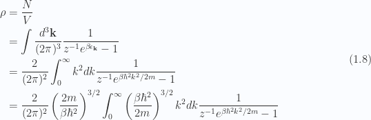

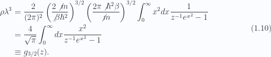


 for the thermal de Broglie wavelength,


 function is plotted in fig. 1.6. The contributions to
  term are dropped for the high temperature approximation.


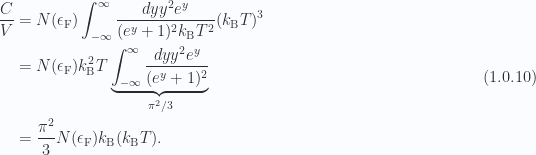
 we have


 is called the degeneracy pressure.


 is approximately constant as in fig. 1.3.


 , so that we have near cancelation of the
  factor
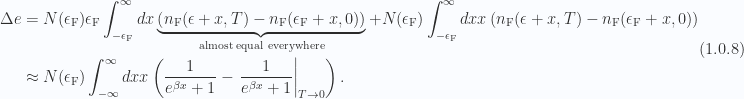
 since this doesn’t change much. FIXME: justify this to myself? Taking derivatives with respect to temperature we have
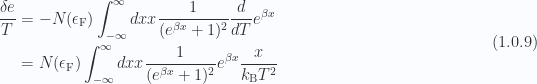
 , we have for


 as illustrated in fig. 1.6.


 . FIXME: that bit wasn’t clear to me.


 are
are  , we have


 . For the low temperature asymptotic behavior see [1] appendix section E. For
  large it can be shown that this is


 for small
  , for an end result of


 and a state in which it is open with energy
  . we require, however, that the zipper can only unzip from the left end, and that the link number
  can only open if all links to the left
  are already open. Find (and sum) the partition function. In the low temperature limit
  , find the average number of open links. The model is a very simplified model of the unwinding of two-stranded DNA molecules.
 and
and  states.
 .
.


 (small
  ), we have
 for a few small

 on
on 


 approximations that we have to use when the number of particles is explicitly fixed.


 , or
, or


 .
.


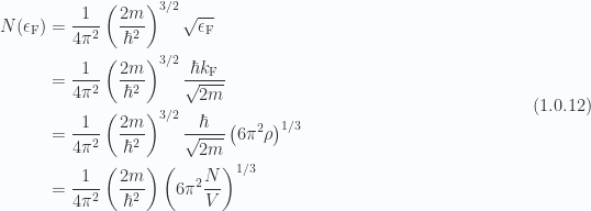
 ) leads us to the desired result
