PHY450H1S. Relativistic Electrodynamics Tutorial 4 (TA: Simon Freedman). Waveguides: confined EM waves.

[Click here for a PDF of this post with nicer formatting]

Motivation

While this isn’t part of the course, the topic of waveguides is one of so many applications that it is worth a mention, and that will be done in this tutorial.

We will setup our system with a waveguide (conducting surface that confines the radiation) oriented in the direction. The shape can be arbitrary

PICTURE: cross section of wacky shape.

At the surface of a conductor.

At the surface of the conductor (I presume this means the interior surface where there is no charge or current enclosed) we have

If we are talking about the exterior surface, do we need to make any other assumptions (perfect conductors, or constant potentials)?

Wave equations.

For electric and magnetic fields in vacuum, we can show easily that these, like the potentials, separately satisfy the wave equation

Taking curls of the Maxwell curl equations above we have

but we have for vector

which gives us a pair of wave equations

We still have the original constraints of Maxwell’s equations to deal with, but we are free now to pick the complex exponentials as fundamental solutions, as our starting point

With and this is

For the vacuum case, with monochromatic light, we treated the amplitudes as constants. Let’s see what happens if we relax this assumption, and allow for spatial dependence (but no time dependence) of and . For the LHS of the electric field curl equation we have

Similarly for the divergence we have

This provides constraints on the amplitudes

Applying the wave equation operator to our phasor we get

So the momentum space equivalents of the wave equations are

Observe that if , then these amplitudes are harmonic functions (solutions to the Laplacian equation). However, it doesn’t appear that we require such a light like relation for the four vector .

Back to the tutorial notes.

In class we went straight to an assumed solution of the form

where . Our Laplacian was also written as the sum of components in the propagation and perpendicular directions

With no dependence in the amplitudes we have

Separation into components.

It was left as an exercise to separate out our Maxwell equations, so that our field components and in the propagation direction, and components in the perpendicular direction are separated

We can do something similar for . This allows for a split of 1.14 into and perpendicular components

So we see that once we have a solution for and (by solving the wave equation above for those components), the components for the fields in terms of those components can be found. Alternately, if one solves for the perpendicular components of the fields, these propagation components are available immediately with only differentiation.

In the case where the perpendicular components are taken as given

we can express the remaining ones strictly in terms of the perpendicular fields

Is it at all helpful to expand the double cross products?

This gives us

but that doesn’t seem particularly useful for completely solving the system? It appears fairly messy to try to solve for and given the propagation direction fields. I wonder if there is a simplification available that I am missing?

Solving the momentum space wave equations.

Back to the class notes. We proceeded to solve for and from the wave equations by separation of variables. We wish to solve equations of the form

Write , so that we have

One solution is sinusoidal

The example in the tutorial now switched to a rectangular waveguide, still oriented with the propagation direction down the z-axis, but with lengths and along the and axis respectively.

Writing , and , we have

We were also provided with some definitions

\begin{definition}TE (Transverse Electric)

.
\end{definition}
\begin{definition}
TM (Transverse Magnetic)

.
\end{definition}
\begin{definition}
TM (Transverse Electromagnetic)

.
\end{definition}

\begin{claim}TEM do not existing in a hollow waveguide.
\end{claim}

Why: I had in my notes

and then

In retrospect I fail to see how these are connected? What happened to the term in the curl equation above?

It was argued that we have on the boundary.

So for the TE case, where , we have from the separation of variables argument

No sines because

The quantity

is called the mode. Note that since an ampere loop requires since there is no current.

Writing

Since we have purely imaginary, and the term

represents the die off.

is the smallest.

Note that the convention is that the in is the bigger of the two indexes, so .

The phase velocity

However, energy is transmitted with the group velocity, the ratio of the Poynting vector and energy density

(This can be shown).

Since

We see that the energy is transmitted at less than the speed of light as expected.

Final remarks.

I’d started converting my handwritten scrawl for this tutorial into an attempt at working through these ideas with enough detail that they self contained, but gave up part way. This appears to me to be too big of a sub-discipline to give it justice in one hours class. As is, it is enough to at least get an concept of some of the ideas involved. I think were I to learn this for real, I’d need a good text as a reference (or the time to attempt to blunder through the ideas in much much more detail).

PHY450H1S. Relativistic Electrodynamics Lecture 11 (Taught by Prof. Erich Poppitz). Unpacking Lorentz force equation. Lorentz transformations of the strength tensor, Lorentz field invariants, Bianchi identity, and first half of Maxwell’s.

[Click here for a PDF of this post with nicer formatting (especially if my latex to wordpress script has left FORMULA DOES NOT PARSE errors.)]

Reading.

Covering chapter 3 material from the text [1].

Covering lecture notes pp. 74-83: Lorentz transformation of the strength tensor (82) [Tuesday, Feb. 8] [extra reading for the mathematically minded: gauge field, strength tensor, and gauge transformations in differential form language, not to be covered in class (83)]

Covering lecture notes pp. 84-102: Lorentz invariants of the electromagnetic field (84-86); Bianchi identity and the first half of Maxwell’s equations (87-90)

Chewing on the four vector form of the Lorentz force equation.

After much effort, we arrived at

or

Elements of the strength tensor

\paragraph{Claim}: there are only 6 independent elements of this matrix (tensor)

This is a no-brainer, for we just have to mechanically plug in the elements of the field strength tensor

Recall

For the purely spatial index combinations we have

Written out explicitly, these are

We can compare this to the elements of

We see that

So we have

These can be summarized as simply

This provides all the info needed to fill in the matrix above

Index raising of rank 2 tensor

To raise indexes we compute

Justifying the raising operation.

To justify this consider raising one index at a time by applying the metric tensor to our definition of . That is

Now apply the metric tensor once more

This is, by definition . Since a rank 2 tensor has been defined as an object that transforms like the product of two pairs of coordinates, it makes sense that this particular tensor raises in the same fashion as would a product of two vector coordinates (in this case, it happens to be an antisymmetric product of two vectors, and one of which is an operator, but we have the same idea).

Consider the components of the raised tensor.

Back to chewing on the Lorentz force equation.

For the spatial components of the Lorentz force equation we have

But

Canceling the common terms, and switching to vector notation, we are left with

Now for the energy term. We have

Putting the final two lines into vector form we have

or

Transformation of rank two tensors in matrix and index form.

Transformation of the metric tensor, and some identities.

With

\paragraph{We claim:}
The rank two tensor transforms in the following sort of sandwich operation, and this leaves it invariant

To demonstrate this let’s consider a transformed vector in coordinate form as follows

We can thus write the equation in matrix form with

Our invariant for the vector square, which is required to remain unchanged is

This shows that we have a delta function relationship for the Lorentz transform matrix, when we sum over the first index

It appears we can put 3.37 into matrix form as

Now, if one considers that the transpose of a rotation is an inverse rotation, and the transpose of a boost leaves it unchanged, the transpose of a general Lorentz transformation, a composition of an arbitrary sequence of boosts and rotations, must also be a Lorentz transformation, and must then also leave the norm unchanged. For the transpose of our Lorentz transformation lets write

For the action of this on our position vector let’s write

so that our norm is

We must then also have an identity when summing over the second index

Armed with these facts on the products of and we can now consider the transformation of the metric tensor.

The rule (definition) supplied to us for the transformation of an arbitrary rank two tensor, is that this transforms as its indexes transform individually. Very much as if it was the product of two coordinate vectors and we transform those coordinates separately. Doing so for the metric tensor we have

However, by 3.42, we have , and we prove that

Finally, we wish to put the above transformation in matrix form, look more carefully at the very first line

which is

We see that this particular form of transformation, a sandwich between and , leaves the metric tensor invariant.

Lorentz transformation of the electrodynamic tensor

Having identified a composition of Lorentz transformation matrices, when acting on the metric tensor, leaves it invariant, it is a reasonable question to ask how this form of transformation acts on our electrodynamic tensor ?

\paragraph{Claim:} A transformation of the following form is required to maintain the norm of the Lorentz force equation

where . Observe that our Lorentz force equation can be written exclusively in upper index quantities as

Because we have a vector on one side of the equation, and it transforms by multiplication with by a Lorentz matrix in SO(1,3)

The LHS of the Lorentz force equation provides us with one invariant

so the RHS must also provide one

Let’s look at the RHS in matrix form. Writing

we can rewrite the Lorentz force equation as

In this matrix formalism our invariant 3.49 is

If we compare this to the transformed Lorentz force equation we have

Our invariant for the transformed equation is

Thus the transformed electrodynamic tensor must satisfy the identity

With the substitution the LHS is

We’ve argued that is also a Lorentz transformation, thus

This is enough to make both sides of 3.54 match, verifying that this transformation does provide the invariant properties desired.

Direct computation of the Lorentz transformation of the electrodynamic tensor.

We can construct the transformed field tensor more directly, by simply transforming the coordinates of the four gradient and the four potential directly. That is

By inspection we can see that this can be represented in matrix form as

Four vector invariants

For three vectors and invariants are

For four vectors and invariants are

For what are the invariants? One invariant is

but this isn’t interesting since it is uniformly zero (product of symmetric and antisymmetric).

The two invariants are

and

where

i j k l=0123$ } \\ -1 & \quad \mbox{for odd permutations of $i j k l=0123$ } \\ \end{array}\right.\end{aligned} \hspace{\stretch{1}}(4.61)$

We can show (homework) that

This first invariant serves as the action density for the Maxwell field equations.

There’s some useful properties of these invariants. One is that if the fields are perpendicular in one frame, then will be in any other.

From the first, note that if , the invariant is positive, and must be positive in all frames, or if in one frame, we can transform to a frame with only component, solve that, and then transform back. Similarly if in one frame, we can transform to a frame with only component, solve that, and then transform back.

The first half of Maxwell’s equations.

\paragraph{Claim: } The source free portions of Maxwell’s equations are a consequence of the definition of the field tensor alone.

Given

where

This alone implies half of Maxwell’s equations. To show this we consider

This is the Bianchi identity. To demonstrate this identity, we’ll have to swap indexes, employ derivative commutation, and then swap indexes once more

This is the 4D analogue of

i.e.

Let’s do this explicitly, starting with

For the case we have

We must then have

This is just Gauss’s law for magnetism

Let’s do the spatial portion, for which we have three equations, one for each of

This implies

Referring back to the previous expansions of 2.6 and 2.17, we have

or

These are just the components of the Maxwell-Faraday equation

Appendix. Some additional index gymnastics.

Transposition of mixed index tensor.

Is the transpose of a mixed index object just a substitution of the free indexes? This wasn’t obvious to me that it would be the case, especially since I’d made an error in some index gymnastics that had me temporarily convinced differently. However, working some examples clears the fog. For example let’s take the transpose of 3.37.

If the transpose of a mixed index tensor just swapped the indexes we would have

From this it does appear that all we have to do is switch the indexes and we will write

We can consider a more general operation

So we see that we do just have to swap indexes.

Transposition of lower index tensor.

We’ve saw above that we had

which followed by careful treatment of the transposition in terms of for which we defined a transpose operation. We assumed as well that

However, this does not have to be assumed, provided that , and . We see this by expanding this transposition in products of and

It would be worthwhile to go through all of this index manipulation stuff and lay it out in a structured axiomatic form. What is the minimal set of assumptions, and how does all of this generalize to non-diagonal metric tensors (even in Euclidean spaces).

Translating the index expression of identity from Lorentz products to matrix form

A verification that the matrix expression 3.38, matches the index expression 3.37 as claimed is worthwhile. It would be easy to guess something similar like is instead the matrix representation. That was in fact my first erroneous attempt to form the matrix equivalent, but is the transpose of 3.38. Either way you get an identity, but the indexes didn’t match.

Since we have which do we pick to do this verification? This appears to be dictated by requirements to match lower and upper indexes on the summed over index. This is probably clearest by example, so let’s expand the products on the LHS explicitly

This matches the that we have on the RHS, and all is well.

References

[1] L.D. Landau and E.M. Lifshitz. The classical theory of fields. Butterworth-Heinemann, 1980.

PHY450H1S. Relativistic Electrodynamics Lecture 14 (Taught by Simon Freedman). Wave equation in Coulomb and Lorentz gauges.

[Click here for a PDF of this post with nicer formatting]

Reading.

Covering chapter 4 material from the text [1].

Covering lecture notes pp.103-114: the wave equation in the relativistic Lorentz gauge (114-114) [Tuesday, Feb. 15; Wednesday, Feb.16]…

Covering lecture notes pp. 114-127: reminder on wave equations (114); reminder on Fourier series and integral (115-117); Fourier expansion of the EM potential in Coulomb gauge and equation of motion for the spatial Fourier components (118-119); the general solution of Maxwell’s equations in vacuum (120-121) [Tuesday, Mar. 1]; properties of monochromatic plane EM waves (122-124); energy and energy flux of the EM field and energy conservation from the equations of motion (125-127) [Wednesday, Mar. 2]

Trying to understand “c”

Maxwell’s equations in a vacuum were

There’s a redundancy here since we can change and without changing the EOM

with

which gives

Maxwell’s equations are now

Can we make , while .

We need

How about

We want the divergence of to be zero, which means

So we want

Can we solve this?

Recall that in electrostatics we have

and

which meant that we had

This has the identical form (with , and ).

While we aren’t trying to actually solve this (just show that it can be solved). One way to look at this problem is that it is just a Laplace equation, and we could utilize a Green’s function solution if desired.

On the Green’s function.

Recall that the Green’s function for the Laplacian was

with the property

Our LDE to solve by Green’s method is

We let this equation (after switching to primed coordinates) operate on the Green’s function

Assuming that the left action of the Green’s function on the test function is the same as the right action (i.e. and commute), we have for the LHS

Substitution of on the RHS then gives us the general solution

Back to Maxwell’s equations in vacuum.

What are the Maxwell’s vacuum equations now?

With the second gauge substitution we have

but we can utilize

to reduce Maxwell’s equations (after dropping primes) to just

where

Note that for this to be correct we have to also explicitly include the gauge condition used. This particular gauge is called the \underline{Coulomb gauge}.

Claim: EM waves propagate with speed and are transverse.

\paragraph{Note:} Is the Coulomb gauge Lorentz invariant?
\paragraph{No.} We can boost which will introduce a non-zero .

The gauge that is Lorentz Invariant is the “Lorentz gauge”. This one uses

Recall that Maxwell’s equations are

where

Writing out the equations in terms of potentials we have

So, if we pick the gauge condition , we are left with just

Can we choose such that ?

Our gauge condition is

Hit it with a derivative for

If we want , then we have

This is the physicist proof. Yes, it can be solved. To really solve this, we’d want to use Green’s functions. I seem to recall the Green’s function is a retarded time version of the Laplacian Green’s function, and we can figure that exact form out by switching to a Fourier frequency domain representation.

Anyways. Returning to Maxwell’s equations we have

where the first is Maxwell’s equation, and the second is our gauge condition.

Observe that the gauge condition is now a Lorentz scalar.

But the Lorentz transform matrices multiply out to identity, in the same way that they do for the transformation of a plain old four vector dot product .

What happens with a Massive vector field?

An aside on units

“Note that this action is expressed in dimensions where , making the action is unit-less (energy and time are inverse units of each other). The has units of (since ), so has units of , and then has units of mass. Therefore has units of and therefore you need something that has units of to make the action unit-less. When you don’t take , then you’ve got to worry about those factors, but I think you’ll see it works out fine.”

For what it’s worth, I can adjust the units of this action to those that we’ve used in class with,

Back to the problem.

The variation of the field invariant is

Variation of the term gives us

so we have

The last integral vanishes on the boundary with the assumption that on that boundary.

Since this must be true for all variations, this leaves us with

The RHS can be expanded into wave equation and divergence parts

With for the wave equation operator

we can manipulate the EOM to pull out an factor

If we hit this with a derivative we get

Since is presumed to be non-zero here, this means that the Lorentz gauge is already chosen for us by the equations of motion.

References

[1] L.D. Landau and E.M. Lifshitz. The classical theory of fields. Butterworth-Heinemann, 1980.

Fourier transform solutions and associated energy and momentum for the homogeneous Maxwell equation. (rework once more)

[Click here for a PDF of this post with nicer formatting]. Note that this PDF file is formatted in a wide-for-screen layout that is probably not good for printing.

These notes build on and replace those formerly posted in Energy and momentum for assumed Fourier transform solutions to the homogeneous Maxwell equation.

Motivation and notation.

In Electrodynamic field energy for vacuum (reworked) [1], building on Energy and momentum for Complex electric and magnetic field phasors [2], a derivation for the energy and momentum density was derived for an assumed Fourier series solution to the homogeneous Maxwell’s equation. Here we move to the continuous case examining Fourier transform solutions and the associated energy and momentum density.

A complex (phasor) representation is implied, so taking real parts when all is said and done is required of the fields. For the energy momentum tensor the Geometric Algebra form, modified for complex fields, is used

The assumed four vector potential will be written

Subject to the requirement that is a solution of Maxwell’s equation

To avoid latex hell, no special notation will be used for the Fourier coefficients,

When convenient and unambiguous, this dependence will be implied.

Having picked a time and space representation for the field, it will be natural to express both the four potential and the gradient as scalar plus spatial vector, instead of using the Dirac basis. For the gradient this is

and for the four potential (or the Fourier transform functions), this is

Setup

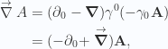
The field bivector is required for the energy momentum tensor. This is

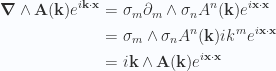
This last term is a spatial curl and the field is then

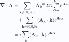
Applied to the Fourier representation this is

It is only the real parts of this that we are actually interested in, unless physical meaning can be assigned to the complete complex vector field.

Constraints supplied by Maxwell’s equation.

A Fourier transform solution of Maxwell’s vacuum equation has been assumed. Having expressed the Faraday bivector in terms of spatial vector quantities, it is more convenient to do this back substitution into after pre-multiplying Maxwell’s equation by , namely

Applied to the spatially decomposed field as specified in (2.7), this is

All grades of this equation must simultaneously equal zero, and the bivector grades have canceled (assuming commuting space and time partials), leaving two equations of constraint for the system

It is immediately evident that a gauge transformation could be immediately helpful to simplify things. In [3] the gauge choice is used. From (3.11) this implies that . Bohm argues that for this current and charge free case this implies , but he also has a periodicity constraint. Without a periodicity constraint it is easy to manufacture non-zero counterexamples. One is a linear function in the space and time coordinates

This is a valid scalar potential provided that the wave equation for the vector potential is also a solution. We can however, force by making the transformation , which in non-covariant notation is

If the transformed field can be forced to zero, then the complexity of the associated Maxwell equations are reduced. In particular, antidifferentiation of , yields

Dropping primes, the transformed Maxwell equations now take the form

There are two classes of solutions that stand out for these equations. If the vector potential is constant in time , Maxwell’s equations are reduced to the single equation

Observe that a gradient can be factored out of this equation

The solutions are then those s that satisfy both

In particular any non-time dependent potential with constant curl provides a solution to Maxwell’s equations. There may be other solutions to (3.19) too that are more general. Returning to (3.17) a second way to satisfy these equations stands out. Instead of requiring of constant curl, constant divergence with respect to the time partial eliminates (3.17). The simplest resulting equations are those for which the divergence is a constant in time and space (such as zero). The solution set are then spanned by the vectors for which

Any that both has constant divergence and satisfies the wave equation will via (2.7) then produce a solution to Maxwell’s equation.

Maxwell equation constraints applied to the assumed Fourier solutions.

Let’s consider Maxwell’s equations in all three forms, (3.11), (3.20), and (3.22) and apply these constraints to the assumed Fourier solution.

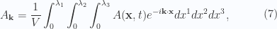
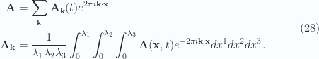
In all cases the starting point is a pair of Fourier transform relationships, where the Fourier transforms are the functions to be determined

Case I. Constant time vector potential. Scalar potential eliminated by gauge transformation.

From (4.24) we require

So the Fourier transform also cannot have any time dependence, and we have

What is the curl of this? Temporarily falling back to coordinates is easiest for this calculation

This gives

We want to equate the divergence of this to zero. Neglecting the integral and constant factor this requires

Requiring that the plane spanned by and be perpendicular to implies that . The solution set is then completely described by functions of the form

where is an arbitrary scalar valued function. This is however, an extremely uninteresting solution since the curl is uniformly zero

Since , when all is said and done the , case appears to have no non-trivial (zero) solutions. Moving on, …

Case II. Constant vector potential divergence. Scalar potential eliminated by gauge transformation.

Next in the order of complexity is consideration of the case (3.22). Here we also have , eliminated by gauge transformation, and are looking for solutions with the constraint

How can this constraint be enforced? The only obvious way is a requirement for to be zero for all , meaning that our to be determined Fourier transform coefficients are required to be perpendicular to the wave number vector parameters at all times.

The remainder of Maxwell’s equations, (3.23) impose the addition constraint on the Fourier transform

For zero equality for all it appears that we require the Fourier transforms to be harmonic in time

This has the familiar exponential solutions

also subject to a requirement that . Our field, where the are to be determined by initial time conditions, is by (2.7) of the form

Since , we have . This allows for factoring out of . The structure of the solution is not changed by incorporating the factors into , leaving the field having the general form

The original meaning of as Fourier transforms of the vector potential is obscured by the tidy up change to absorb , but the geometry of the solution is clearer this way.

It is also particularly straightforward to confirm that separately for either half of (4.34).

Case III. Non-zero scalar potential. No gauge transformation.

Now lets work from (3.11). In particular, a divergence operation can be factored from (3.11), for

Right off the top, there is a requirement for

In terms of the Fourier transforms this is

Are there any ways for this to equal a constant for all without requiring that constant to be zero? Assuming no for now, and that this constant must be zero, this implies a coupling between the and Fourier transforms of the form

A secondary implication is that or else is not a scalar. We had a transverse solution by requiring via gauge transformation that , and here we have instead the vector potential in the propagation direction.

A secondary confirmation that this is a required coupling between the scalar and vector potential can be had by evaluating the divergence equation of (4.35)

Rearranging this also produces (4.38). We want to now substitute this relationship into (3.12).

Starting with just the part we have

Taking the gradient of this brings down a factor of for

(3.12) in its entirety is now

This isn’t terribly pleasant looking. Perhaps going the other direction. We could write

so that

Note that the gradients here operate on everything to the right, including and especially the exponential. Each application of the gradient brings down an additional factor, and we have

This is identically zero, so we see that this second equation provides no additional information. That is somewhat surprising since there is not a whole lot of constraints supplied by the first equation. The function can be anything. Understanding of this curiosity comes from computation of the Faraday bivector itself. From (2.7), that is

All terms cancel, so we see that a non-zero leads to , as was the case when considering (4.24) (a case that also resulted in ).

Can this Fourier representation lead to a non-transverse solution to Maxwell’s equation? If so, it is not obvious how.

The energy momentum tensor

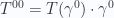
The energy momentum tensor is then

Observing that commutes with spatial bivectors and anticommutes with spatial vectors, and writing , the tensor splits neatly into scalar and spatial vector components

In particular for , we have

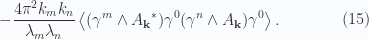
Integrating this over all space and identification of the delta function

reduces the tensor to a single integral in the continuous angular wave number space of .

Or,

Multiplying out (5.53) yields for

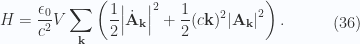
Recall that the only non-trivial solution we found for the assumed Fourier transform representation of was for , . Thus we have for the energy density integrated over all space, just

Observe that we have the structure of a Harmonic oscillator for the energy of the radiation system. What is the canonical momentum for this system? Will it correspond to the Poynting vector, integrated over all space?

Let’s reduce the vector component of (5.53), after first imposing the , and conditions used to above for our harmonic oscillator form energy relationship. This is

This is just

Recall that the Fourier transforms for the transverse propagation case had the form , where the minus generated the advanced wave, and the plus the receding wave. With substitution of the vector potential for the advanced wave into the energy and momentum results of (5.55) and (5.56) respectively, we have

After a somewhat circuitous route, this has the relativistic symmetry that is expected. In particular the for the complete tensor we have after integration over all space

The receding wave solution would give the same result, but directed as instead.

Observe that we also have the four divergence conservation statement that is expected

This follows trivially since both the derivatives are zero. If the integration region was to be more specific instead of a relationship, we’d have the power flux equal in magnitude to the momentum change through a bounding surface. For a more general surface the time and spatial dependencies shouldn’t necessarily vanish, but we should still have this radiation energy momentum conservation.

References

[1] Peeter Joot. Electrodynamic field energy for vacuum. [online]. http://sites.google.com/site/peeterjoot/math2009/fourierMaxVac.pdf.

[2] Peeter Joot. {Energy and momentum for Complex electric and magnetic field phasors.} [online]. http://sites.google.com/site/peeterjoot/math2009/complexFieldEnergy.pdf.

[3] D. Bohm. Quantum Theory. Courier Dover Publications, 1989.

Energy and momentum for assumed Fourier transform solutions to the homogeneous Maxwell equation.

[Click here for a PDF of this post with nicer formatting]

Motivation and notation.

In Electrodynamic field energy for vacuum (reworked) [1], building on Energy and momentum for Complex electric and magnetic field phasors [2] a derivation for the energy and momentum density was derived for an assumed Fourier series solution to the homogeneous Maxwell’s equation. Here we move to the continuous case examining Fourier transform solutions and the associated energy and momentum density.

A complex (phasor) representation is implied, so taking real parts when all is said and done is required of the fields. For the energy momentum tensor the Geometric Algebra form, modified for complex fields, is used

The assumed four vector potential will be written

Subject to the requirement that is a solution of Maxwell’s equation

To avoid latex hell, no special notation will be used for the Fourier coefficients,

When convenient and unambiguous, this dependence will be implied.

Having picked a time and space representation for the field, it will be natural to express both the four potential and the gradient as scalar plus spatial vector, instead of using the Dirac basis. For the gradient this is

and for the four potential (or the Fourier transform functions), this is

Setup

The field bivector is required for the energy momentum tensor. This is

This last term is a spatial curl and the field is then

Applied to the Fourier representation this is

The energy momentum tensor is then

The tensor integrated over all space. Energy and momentum?

Integrating this over all space and identification of the delta function

reduces the tensor to a single integral in the continuous angular wave number space of .

Observing that commutes with spatial bivectors and anticommutes with spatial vectors, and writing , one has

The scalar and spatial vector grade selection operator has been added for convenience and does not change the result since those are necessarily the only grades anyhow. The post multiplication by the observer frame time basis vector serves to separate the energy and momentum like components of the tensor nicely into scalar and vector aspects. In particular for , one could write

If these are correctly identified with energy and momentum then it also ought to be true that we have the conservation relationship

However, multiplying out (3.12) yields for

The vector component takes a bit more work to reduce

Canceling and regrouping leaves

This has no explicit dependence, so the conservation relation (3.14) is violated unless . There is no reason to assume that will be the case. In the discrete Fourier series treatment, a gauge transformation allowed for elimination of , and this implied or constant. We will probably have a similar result here, eliminating most of the terms in (3.15) and (3.16). Except for the constant solution of the field equations there is no obvious way that such a simplified energy expression will have zero derivative.

A more reasonable conclusion is that this approach is flawed. We ought to be looking at the divergence relation as a starting point, and instead of integrating over all space, instead employing Gauss’s theorem to convert the divergence integral into a surface integral. Without math, the conservation relationship probably ought to be expressed as energy change in a volume is matched by the momentum change through the surface. However, without an integral over all space, we do not get the nice delta function cancellation observed above. How to proceed is not immediately clear. Stepping back to review applications of Gauss’s theorem is probably a good first step.

References

[1] Peeter Joot. Electrodynamic field energy for vacuum. [online]. http://sites.google.com/site/peeterjoot/math2009/fourierMaxVac.pdf.

[2] Peeter Joot. {Energy and momentum for Complex electric and magnetic field phasors.} [online]. http://sites.google.com/site/peeterjoot/math2009/complexFieldEnergy.pdf.

Electrodynamic field energy for vacuum (reworked)

[Click here for a PDF of this post with nicer formatting]

Previous version.

This is a reworked version of a previous post ([also in PDF]

Reducing the products in the Dirac basis makes life more complicated then it needs to be (became obvious when attempting to derive an expression for the Poynting integral).

Motivation.

From Energy and momentum for Complex electric and magnetic field phasors [PDF] how to formulate the energy momentum tensor for complex vector fields (ie. phasors) in the Geometric Algebra formalism is now understood. To recap, for the field , where and may be complex vectors we have for Maxwell’s equation

This is a doubly complex representation, with the four vector pseudoscalar acting as a non-commutatitive imaginary, as well as real and imaginary parts for the electric and magnetic field vectors. We take the real part (not the scalar part) of any bivector solution of Maxwell’s equation as the actual solution, but allow ourself the freedom to work with the complex phasor representation when convenient. In these phasor vectors, the imaginary , as in , is a commuting imaginary, commuting with all the multivector elements in the algebra.

The real valued, four vector, energy momentum tensor was found to be

To supply some context that gives meaning to this tensor the associated conservation relationship was found to be

and in particular for , this four vector divergence takes the form

relating the energy term and the Poynting spatial vector with the current density and electric field product that constitutes the energy portion of the Lorentz force density.

Let’s apply this to calculating the energy associated with the field that is periodic within a rectangular prism as done by Bohm in [2]. We do not necessarily need the Geometric Algebra formalism for this calculation, but this will be a fun way to attempt it.

Setup

Let’s assume a Fourier representation for the four vector potential for the field . That is

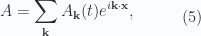
where summation is over all angular wave number triplets . The Fourier coefficients are allowed to be complex valued, as is the resulting four vector , and the associated bivector field .

Fourier inversion, with , follows from

but only this orthogonality relationship and not the Fourier coefficients themselves

will be of interest here. Evaluating the curl for this potential yields

Since the four vector potential has been expressed using an explicit split into time and space components it will be natural to re express the bivector field in terms of scalar and (spatial) vector potentials, with the Fourier coefficients. Writing for the spatial basis vectors, , and , this is

The Faraday bivector field is then

This is now enough to express the energy momentum tensor

It will be more convenient to work with a scalar plus bivector (spatial vector) form of this tensor, and right multiplication by produces such a split

The primary object of this treatment will be consideration of the components of the tensor, which provide a split into energy density , and Poynting vector (momentum density) .

Our first step is to integrate (12) over the volume . This integration and the orthogonality relationship (6), removes the exponentials, leaving

Because commutes with the spatial bivectors, and anticommutes with the spatial vectors, the remainder of the Dirac basis vectors in these expressions can be eliminated

Expanding the energy momentum tensor components.

Energy

In (15) only the bivector-bivector and vector-vector products produce any scalar grades. Except for the bivector product this can be done by inspection. For that part we utilize the identity

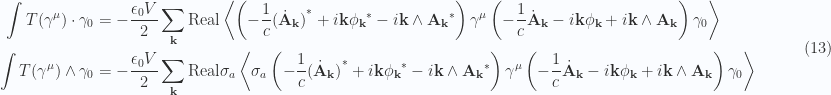
This leaves for the energy in the volume

We are left with a completely real expression, and one without any explicit Geometric Algebra. This does not look like the Harmonic oscillator Hamiltonian that was expected. A gauge transformation to eliminate and an observation about when equals zero will give us that, but first lets get the mechanical jobs done, and reduce the products for the field momentum.

Momentum

Now move on to (16). For the factors other than only the vector-bivector products can contribute to the scalar product. We have two such products, one of the form

and the other

The momentum in this volume follows by computation of

All the products are paired in nice conjugates, taking real parts, and premultiplication with gives the desired result. Observe that two of these terms cancel, and another two have no real part. Those last are

Taking the real part of this pure imaginary is zero, leaving just

I am not sure why exactly, but I actually expected a term with , quadratic in the vector potential. Is there a mistake above?

Gauge transformation to simplify the Hamiltonian.

In (20) something that looked like the Harmonic oscillator was expected. On the surface this does not appear to be such a beast. Exploitation of gauge freedom is required to make the simplification that puts things into the Harmonic oscillator form.

If we are to change our four vector potential , then Maxwell’s equation takes the form

which is unchanged by the addition of the gradient to any original potential solution to the equation. In coordinates this is a transformation of the form

and we can use this to force any one of the potential coordinates to zero. For this problem, it appears that it is desirable to seek a such that . That is

Or,

With such a transformation, the and cross term in the Hamiltonian (20) vanishes, as does the term in the four vector square of the last term, leaving just

Additionally, wedging (5) with now does not loose any information so our potential Fourier series is reduced to just

The desired harmonic oscillator form would be had in (26) if it were not for the term. Does that vanish? Returning to Maxwell’s equation should answer that question, but first it has to be expressed in terms of the vector potential. While , the lack of an component means that this can be inverted as

The gradient can also be factored scalar and spatial vector components

So, with this gauge choice the bivector field is

From the left the gradient action on is

and from the right

Taking the difference we have

Which is just

For this vacuum case, premultiplication of Maxwell’s equation by gives

The spatial bivector and trivector grades are all zero. Equating the remaining scalar and vector components to zero separately yields a pair of equations in

If the divergence of the vector potential is constant we have just a wave equation. Let’s see what that divergence is with the assumed Fourier representation

Since , there are two ways for . For each there must be a requirement for either or . The constant solution to the first equation appears to represent a standing spatial wave with no time dependence. Is that of any interest?

The more interesting seeming case is where we have some non-static time varying state. In this case, if , the second of these Maxwell’s equations is just the vector potential wave equation, since the divergence is zero. That is

Solving this isn’t really what is of interest, since the objective was just to determine if the divergence could be assumed to be zero. This shows then, that if the transverse solution to Maxwell’s equation is picked, the Hamiltonian for this field, with this gauge choice, becomes

How does the gauge choice alter the Poynting vector? From (21), all the dependence in that integrated momentum density is lost

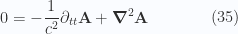
The solutions to Maxwell’s equation are seen to result in zero momentum for this infinite periodic field. My expectation was something of the form , so intuition is either failing me, or my math is failing me, or this contrived periodic field solution leads to trouble.

Conclusions and followup.

The objective was met, a reproduction of Bohm’s Harmonic oscillator result using a complex exponential Fourier series instead of separate sine and cosines.

The reason for Bohm’s choice to fix zero divergence as the gauge choice upfront is now clear. That automatically cuts complexity from the results. Figuring out how to work this problem with complex valued potentials and also using the Geometric Algebra formulation probably also made the work a bit more difficult since blundering through both simultaneously was required instead of just one at a time.

This was an interesting exercise though, since doing it this way I am able to understand all the intermediate steps. Bohm employed some subtler argumentation to eliminate the scalar potential upfront, and I have to admit I did not follow his logic, whereas blindly following where the math leads me all makes sense.

As a bit of followup, I’d like to consider the constant case in more detail, and any implications of the freedom to pick .

The general calculation of for the assumed Fourier solution should be possible too, but was not attempted. Doing that general calculation with a four dimensional Fourier series is likely tidier than working with scalar and spatial variables as done here.

Now that the math is out of the way (except possibly for the momentum which doesn’t seem right), some discussion of implications and applications is also in order. My preference is to let the math sink-in a bit first and mull over the momentum issues at leisure.

References

[2] D. Bohm. Quantum Theory. Courier Dover Publications, 1989.

Electrodynamic field energy for vacuum.

[Click here for a PDF of this post with nicer formatting]

Motivation.

We now know how to formulate the energy momentum tensor for complex vector fields (ie. phasors) in the Geometric Algebra formalism. To recap, for the field , where and may be complex vectors we have for Maxwell’s equation

This is a doubly complex representation, with the four vector pseudoscalar acting as a non-commutatitive imaginary, as well as real and imaginary parts for the electric and magnetic field vectors. We take the real part (not the scalar part) of any bivector solution of Maxwell’s equation as the actual solution, but allow ourself the freedom to work with the complex phasor representation when convenient. In these phasor vectors, the imaginary , as in , is a commuting imaginary, commuting with all the multivector elements in the algebra.

The real valued, four vector, energy momentum tensor was found to be

To supply some context that gives meaning to this tensor the associated conservation relationship was found to be

and in particular for , this four vector divergence takes the form

relating the energy term and the Poynting spatial vector with the current density and electric field product that constitutes the energy portion of the Lorentz force density.

Let’s apply this to calculating the energy associated with the field that is periodic within a rectangular prism as done by Bohm in [1]. We do not necessarily need the Geometric Algebra formalism for this calculation, but this will be a fun way to attempt it.

Setup

Let’s assume a Fourier representation for the four vector potential for the field . That is

where summation is over all wave number triplets . The Fourier coefficients are allowed to be complex valued, as is the resulting four vector , and the associated bivector field .

Fourier inversion follows from

but only this orthogonality relationship and not the Fourier coefficients themselves

will be of interest here. Evaluating the curl for this potential yields

We can now form the energy density

With implied summation over all repeated integer indexes (even without matching uppers and lowers), this is

The grade selection used here doesn’t change the result since we already have a scalar, but will just make it convenient to filter out any higher order products that will cancel anyways. Integrating over the volume element and taking advantage of the orthogonality relationship (6), the exponentials are removed, leaving the energy contained in the volume

First reduction of the Hamiltonian.

Let’s take the products involved in sequence one at a time, and evaluate, later adding and taking real parts if required all of

The expectation is to obtain a Hamiltonian for the field that has the structure of harmonic oscillators, where the middle two products would have to be zero or sum to zero or have real parts that sum to zero. The first is expected to contain only products of , and the last only products of .

While initially guessing that (13) and (14) may cancel, this isn’t so obviously the case. The use of cyclic permutation of multivectors within the scalar grade selection operator plus a change of dummy summation indexes in one of the two shows that this sum is of the form . This sum is intrinsically real, so we can neglect one of the two doubling the other, but we will still be required to show that the real part of either is zero.

Lets reduce these one at a time starting with (12), and write temporarily

So the first of our Hamiltonian terms is

Note that summation over is still implied here, so we’d be better off with a spatial vector representation of the Fourier coefficients . With such a notation, this contribution to the Hamiltonian is

To reduce (13) and (13), this time writing , we can start with just the scalar selection

Thus the contribution to the Hamiltonian from (13) and (13) is

Most definitively not zero in general. Our final expansion (15) is the messiest. Again with for short, the grade selection of this term in coordinates is

Expanding this out yields

The contribution to the Hamiltonian from this, with , is then

A final reassembly of the Hamiltonian from the parts (17) and (18) and (21) is then

This is finally reduced to a completely real expression, and one without any explicit Geometric Algebra. All the four vector Fourier vector potentials written out explicitly in terms of the spacetime split , which is natural since an explicit time and space split was the starting point.

Gauge transformation to simplify the Hamiltonian.

While (22) has considerably simpler form than (11), what was expected, was something that looked like the Harmonic oscillator. On the surface this does not appear to be such a beast. Exploitation of gauge freedom is required to make the simplification that puts things into the Harmonic oscillator form.

If we are to change our four vector potential , then Maxwell’s equation takes the form

which is unchanged by the addition of the gradient to any original potential solution to the equation. In coordinates this is a transformation of the form

and we can use this to force any one of the potential coordinates to zero. For this problem, it appears that it is desirable to seek a such that . That is

Or,

With such a transformation, the and cross term in the Hamiltonian (22) vanishes, as does the term in the four vector square of the last term, leaving just

Additionally, wedging (5) with now does not loose any information so our potential Fourier series is reduced to just

The desired harmonic oscillator form would be had in (27) if it were not for the term. Does that vanish? Returning to Maxwell’s equation should answer that question, but first it has to be expressed in terms of the vector potential. While , the lack of an component means that this can be inverted as

The gradient can also be factored scalar and spatial vector components

So, with this gauge choice the bivector field is

From the left the gradient action on is

and from the right

Taking the difference we have

Which is just

For this vacuum case, premultiplication of Maxwell’s equation by gives

The spatial bivector and trivector grades are all zero. Equating the remaining scalar and vector components to zero separately yields a pair of equations in

If the divergence of the vector potential is constant we have just a wave equation. Let’s see what that divergence is with the assumed Fourier representation

Since , there are two ways for . For each there must be a requirement for either or . The constant solution to the first equation appears to represent a standing spatial wave with no time dependence. Is that of any interest?

The more interesting seeming case is where we have some non-static time varying state. In this case, if for all the second of these Maxwell’s equations is just the vector potential wave equation, since the divergence is zero. That is

Solving this isn’t really what is of interest, since the objective was just to determine if the divergence could be assumed to be zero. This shows then, that if the transverse solution to Maxwell’s equation is picked, the Hamiltonian for this field, with this gauge choice, becomes

Conclusions and followup.

The objective was met, a reproduction of Bohm’s Harmonic oscillator result using a complex exponential Fourier series instead of separate sine and cosines.

The reason for Bohm’s choice to fix zero divergence as the gauge choice upfront is now clear. That automatically cuts complexity from the results. Figuring out how to work this problem with complex valued potentials and also using the Geometric Algebra formulation probably also made the work a bit more difficult since blundering through both simultaneously was required instead of just one at a time.

This was an interesting exercise though, since doing it this way I am able to understand all the intermediate steps. Bohm employed some subtler argumentation to eliminate the scalar potential upfront, and I have to admit I did not follow his logic, whereas blindly following where the math leads me all makes sense.

As a bit of followup, I’d like to consider the constant case, and any implications of the freedom to pick . I’d also like to construct the Poynting vector , and see what the structure of that is with this Fourier representation.

A general calculation of for an assumed Fourier solution should be possible too, but working in spatial quantities for the general case is probably torture. A four dimensional Fourier series is likely a superior option for the general case.

References

[1] D. Bohm. Quantum Theory. Courier Dover Publications, 1989.

Energy and momentum for Complex electric and magnetic field phasors.

[Click here for a PDF of this post with nicer formatting]

Motivation.

In [1] a complex phasor representations of the electric and magnetic fields is used

Here the vectors and are allowed to take on complex values. Jackson uses the real part of these complex vectors as the true fields, so one is really interested in just these quantities

but carry the whole thing in manipulations to make things simpler. It is stated that the energy for such complex vector fields takes the form (ignoring constant scaling factors and units)

In some ways this is an obvious generalization. Less obvious is how this and the Poynting vector are related in their corresponding conservation relationships.

Here I explore this, employing a Geometric Algebra representation of the energy momentum tensor based on the real field representation found in [2]. Given the complex valued fields and a requirement that both the real and imaginary parts of the field satisfy Maxwell’s equation, it should be possible to derive the conservation relationship between the energy density and Poynting vector from first principles.

Review of GA formalism for real fields.

In SI units the Geometric algebra form of Maxwell’s equation is

where one has for the symbols

The symmetric electrodynamic energy momentum tensor for real fields and is

It may not be obvious that this is in fact a four vector, but this can be seen since it can only have grade one and three components, and also equals its reverse implying that the grade three terms are all zero. To illustrate this explicitly consider the components of

Our result is a four vector in the Dirac basis as expected

Similar expansions are possible for the general tensor components but lets defer this more general expansion until considering complex valued fields. The main point here is to remind oneself how to express the energy momentum tensor in a fashion that is natural in a GA context. We also know that one has a conservation relationship associated with the divergence of this tensor (ie. ), and want to rederive this relationship after guessing what form the GA expression for the energy momentum tensor takes when one allows the field vectors to take complex values.

Computing the conservation relationship for complex field vectors.

As in 5, if one wants

it is reasonable to assume that our energy momentum tensor will take the form

For real vector fields this reduces to the previous results and should produce the desired mix of real and imaginary dot products for the energy density term of the tensor. This is also a real four vector even when the field is complex, so the energy density and power density terms will all be real valued, which seems desirable.

Expanding the tensor. Easy parts.

As with real fields expansion of in terms of and is simplest for . Let’s start with that.

This gives

The sum of and its conjugate has produced the desired energy density expression. An implication of this is that one can form and take real parts of a complex Poynting vector to calculate the momentum density. This is stated but not demonstrated in Jackson, perhaps considered too obvious or messy to derive.

Observe that the a choice to work with complex valued vector fields gives a nice consistency, and one has the same factor of in both the energy and momentum terms. While the energy term is obviously real, the momentum terms can be written in an explicitly real notation as well since one has a quantity plus its conjugate. Using a more conventional four vector notation (omitting the explicit Dirac basis vectors), one can write this out as a strictly real quantity.

Observe that when the vector fields are restricted to real quantities, the conjugate and real part operators can be dropped and the real vector field result 16 is recovered.

Expanding the tensor. Messier parts.

I intended here to compute , and my starting point was a decomposition of the field vectors into components that anticommute or commute with

The components parallel to the spatial vector are anticommuting , whereas the perpendicular components commute . The expansion of the tensor products is then

This isn’t particularly pretty to expand out. I did attempt it, but my result looked wrong. For the application I have in mind I do not actually need anything more than , so rather than show something wrong, I’ll just omit it (at least for now).

Calculating the divergence.

Working with 20, let’s calculate the divergence and see what one finds for the corresponding conservation relationship.

We have then for the divergence

Lets write out in the (stationary) observer frame where . This is

Writing out the four divergence relationships in full one has

Just as in the real field case one has a nice relativistic split into energy density and force (momentum change) components, but one has to take real parts and conjugate half the terms appropriately when one has complex fields.

Combining the divergence relation for with 22 the conservation relation for this subset of the energy momentum tensor becomes

Or

It is this last term that puts some meaning behind Jackson’s treatment since we now know how the energy and momentum are related as a four vector quantity in this complex formalism.

While I’ve used geometric algebra to get to this final result, I would be interested to compare how the intermediate mess compares with the same complex field vector result obtained via traditional vector techniques. I am sure I could try this myself, but am not interested enough to attempt it.

Instead, now that this result is obtained, proceeding on to application is now possible. My intention is to try the vacuum electromagnetic energy density example from [3] using complex exponential Fourier series instead of the doubled sum of sines and cosines that Bohm used.

References

[1] JD Jackson. Classical Electrodynamics Wiley. 2nd edition, 1975.

[2] C. Doran and A.N. Lasenby. Geometric algebra for physicists. Cambridge University Press New York, Cambridge, UK, 1st edition, 2003.

[3] D. Bohm. Quantum Theory. Courier Dover Publications, 1989.

Electromagnetic Gauge invariance.

[Click here for a PDF of this post with nicer formatting]

At the end of section 12.1 in Jackson [1] he states that it is obvious that the Lorentz force equations are gauge invarient.

Since I didn’t remember what Gauge invariance was, it wasn’t so obvious. But if I looking ahead to one of the problem 12.2 on this invariance we have a Gauge transformation defined in four vector form as

In vector form with , this gauge transformation can be written

so this is really a statement that we add a spacetime gradient of something to the four vector potential. Given this, how does the field transform?

But (assuming partials are interchangable) so the field is invariant regardless of whether we are talking about the Lorentz force

or the field equations themselves

So, once you know the definition of the gauge transformation in four vector form, yes this justifiably obvious, however, to anybody who is not familiar with Geometric Algebra, perhaps this is still not so obvious. How does this translate to the more common place tensor or space time vector notations? The tensor four vector translation is the easier of the two, and there we have

As required for interchange of partials means the field components are unchanged by adding this gradient. Finally, in plain old spatial vector form, how is this gauge invariance expressed?

In components we have

This last in vector form is , where the sign inversion comes from , assuming a metric.

We want to apply this to the electric and magnetic field components

The electric field transforms as

With partial interchange this is just . For the magnetic field we have

Again since the partials interchange we have , so this is just the magnetic field.

Alright. Worked this in three different ways, so now I can say its obvious.

References

[1] JD Jackson. Classical Electrodynamics Wiley. 2nd edition, 1975.

Relativistic classical proton electron interaction. (a start).

[Click here for a PDF of this sequence of posts with nicer formatting]

Motivation

The problem of a solving for the relativistically correct trajectories of classically interacting proton and electron is one that I’ve wanted to try for a while. Conceptually this is just about the simplest interaction problem in electrodynamics (other than motion of a particle in a field), but it is not obvious to me how to even set up the right equations to solve. I should have the tools now to at least write down the equations to solve, and perhaps solve them too.

Familiarity with Geometric Algebra, and the STA form of the Maxwell and Lorentz force equation will be assumed. Writing for the Faraday bivector, these equations are respectively

The possibility of self interaction will also be ignored here. From what I have read this self interaction is more complex than regular two particle interaction.

With only Coulomb interaction.

With just Coulomb (non-relativistic) interaction setup of the equations of motion for the relative vector difference between the particles is straightforward. Let’s write this out as a reference. Whatever we come up with for the relativistic case should reduce to this at small velocities.

Fixing notation, lets write the proton and electron positions respectively by and , the proton charge as , and the electron charge . For the forces we have

FIXME: picture

Subtracting the two after mass division yields the reduced mass equation for the relative motion

This is now of the same form as the classical problem of two particle gravitational interaction, with the well known conic solutions.

Using the divergence equation instead.

While use of the Coulomb force above provides the equation of motion for the relative motion of the charges, how to generalize this to the relativistic case is not entirely clear. For the relativistic case we need to consider all of Maxwell’s equations, and not just the divergence equation. Let’s back up a step and setup the problem using the divergence equation instead of Coulomb’s law. This is a bit closer to the use of all of Maxwell’s equations.

To start off we need a discrete charge expression for the charge density, and can use the delta distribution to express this.

Picking a volume element that only encloses one of the respective charges gives us the Coulomb law for the field produced by those charges as above

Here and denote the electric fields due to the proton and electron respectively. Ignoring the possibility of self interaction the Lorentz forces on the particles are

In symbols, this is

If we were to substitute back into the volume integrals we’d have

It is tempting to take the differences of these two equations so that we can write this in terms of the relative acceleration . I did just this initially, and was surprised by a mass term of the form instead of reduced mass, which cannot be right. The key to avoiding this mistake is the proper considerations of the integration volumes. Since the volumes are different and can in fact be entirely disjoint, subtracting these is not possible. For this reason we have to be especially careful if a differential form of the divergence integrals (9) were to be used, as in

The domain of applicability of these equations is no longer explicit, since each has to omit a neighborhood around the other charge. When using a delta distribution to express the point charge density it is probably best to stick with an explicit integral form.

Comparing how far we can get starting with the Gauss’s law instead of the Coulomb force, and looking forward to the relativistic case, it seems likely that solving the field equations due to the respective current densities will be the first required step. Only then can we substitute that field solution back into the Lorentz force equation to complete the search for the particle trajectories.

Relativistic interaction.

First order of business is an expression for a point charge current density four vector. Following Jackson [1], but switching to vector notation from coordinates, we can apparently employ an arbitrary parametrization for the four-vector particle trajectory , as measured in the observer frame, and write

Here is the four vector event specifying the spacetime position of the current, also as measured in the observer frame. Reparameterizating in terms of time should get us back something more familiar looking

Note that the scaling property of the delta function implies . With the split of the four-volume delta function , where , we have an explanation for why Jackson had a factor of in his representation. I initially thought this factor of was due to CGS vs SI units! One more Jackson equation decoded. We are left with the following spacetime split for a point charge current density four vector

Comparing to the continuous case where we have , it appears that this works out right. One thing worth noting is that in this time reparameterization I accidentally mixed up , the observation event coordinates of , and , the spacetime trajectory of the particle itself. Despite this, I am saved by the delta function since no contributions to the current can occur on trajectories other than , the worldline of the particle itself. So in the final result it should be correct to interpret as the spatial particle velocity as I did accidentally.

With the time reparameterization of the current density, we have for the field due to our proton and electron

How to write this in a more tidy covariant form? If we reparametrize with any of the other spatial coordinates, say we end up having to integrate the field gradient with a spacetime three form ( if parametrizing the current density with ). Since the entire equation must be zero I suppose we can just integrate that once more, and simply write

Like (7) we can pick spacetime volumes that surround just the individual particle worldlines, in which case we have a Coulomb’s law like split where the field depends on just the enclosed current. That is

Here is the field due to only the electron charge, whereas would be that part of the total field due to the proton charge.

FIXME: attempt to draw a picture (one or two spatial dimensions) to develop some comfort with tossing out a phrase like “spacetime volume surrounding a particle worldline”.

Having expressed the equation for the total field (18), we are tracking a nice parallel to the setup for the non-relativistic treatment. Next is the pair of Lorentz force equations. As in the non-relativistic setup, if we only consider the field due to the other charge we have in
in covariant Geometric Algebra form, the following pair of proper force equations in terms of the particle worldline trajectories

We have the four sets of coupled multivector equations to be solved, so the question remains how to do so. Each of the two Lorentz force equations supplies four equations with four unknowns, and the field equations are really two sets of eight equations with six unknown field variables each. Then they are all tied up together is a big coupled mess. Wow. How do we solve this?

With (19), and (21) committed to pdf at least the first goal of writing down the equations is done.

As for the actual solution. Well, that’s a problem for another night. TO BE CONTINUED (if I can figure out an attack).

References

[1] JD Jackson. Classical Electrodynamics Wiley. 2nd edition, 1975.

[2] C. Doran and A.N. Lasenby. Geometric algebra for physicists. Cambridge University Press New York, Cambridge, UK, 1st edition, 2003.