Peeter Joot's (OLD) Blog.

Math, physics, perl, and programming obscurity.

Posts Tagged ‘gradient’

Stokes theorem in Geometric algebra

Posted by peeterjoot on May 17, 2014

[Click here for a PDF of this post with nicer formatting  (especially since my latex to wordpress script has left FORMULA DOES NOT PARSE errors.)]

Understanding how to apply Stokes theorem to higher dimensional spaces, non-Euclidean metrics, and with curvilinear coordinates has been a long standing goal.

A traditional answer to these questions can be found in the formalism of differential forms, as covered for example in [2], and [8]. However, both of those texts, despite their small size, are intensely scary. I also found it counter intuitive to have to express all physical quantities as forms, since there are many times when we don’t have any pressing desire to integrate these.

Later I encountered Denker’s straight wire treatment [1], which states that the geometric algebra formulation of Stokes theorem has the form

\begin{aligned}\int_S \nabla \wedge F = \int_{\partial S} F\end{aligned} \hspace{\stretch{1}}(1.0.1)

This is simple enough looking, but there are some important details left out. In particular the grades do not match, so there must be some sort of implied projection or dot product operations too. We also need to understand how to express the hypervolume and hypersurfaces when evaluating these integrals, especially when we want to use curvilinear coordinates.

I’d attempted to puzzle through these details previously. A collection of these attempts, to be removed from my collection of geometric algebra notes, can be found in [4]. I’d recently reviewed all of these and wrote a compact synopsis [5] of all those notes, but in the process of doing so, I realized there was a couple of fundamental problems with the approach I had used.

One detail that was that I failed to understand, was that we have a requirement for treating a infinitesimal region in the proof, then summing over such regions to express the boundary integral. Understanding that the boundary integral form and its dot product are both evaluated only at the end points of the integral region is an important detail that follows from such an argument (as used in proof of Stokes theorem for a 3D Cartesian space in [7].)

I also realized that my previous attempts could only work for the special cases where the dimension of the integration volume also equaled the dimension of the vector space. The key to resolving this issue is the concept of the tangent space, and an understanding of how to express the projection of the gradient onto the tangent space. These concepts are covered thoroughly in [6], which also introduces Stokes theorem as a special case of a more fundamental theorem for integration of geometric algebraic objects. My objective, for now, is still just to understand the generalization of Stokes theorem, and will leave the fundamental theorem of geometric calculus to later.

Now that these details are understood, the purpose of these notes is to detail the Geometric algebra form of Stokes theorem, covering its generalization to higher dimensional spaces and non-Euclidean metrics (i.e. especially those used for special relativity and electromagnetism), and understanding how to properly deal with curvilinear coordinates. This generalization has the form

Theorem 1. Stokes’ Theorem

For blades F \in \bigwedge^{s}, and m volume element d^k \mathbf{x}, s < k,

\begin{aligned}\int_V d^k \mathbf{x} \cdot (\boldsymbol{\partial} \wedge F) = \int_{\partial V} d^{k-1} \mathbf{x} \cdot F.\end{aligned}

Here the volume integral is over a m dimensional surface (manifold), \boldsymbol{\partial} is the projection of the gradient onto the tangent space of the manifold, and \partial V indicates integration over the boundary of V.

It takes some work to give this more concrete meaning. I will attempt to do so in a gradual fashion, and provide a number of examples that illustrate some of the relevant details.

Basic notation

A finite vector space, not necessarily Euclidean, with basis \left\{ {\mathbf{e}_1, \mathbf{e}_2, \cdots} \right\} will be assumed to be the generator of the geometric algebra. A dual or reciprocal basis \left\{ {\mathbf{e}^1, \mathbf{e}^2, \cdots} \right\} for this basis can be calculated, defined by the property

\begin{aligned}\mathbf{e}_i \cdot \mathbf{e}^j = {\delta_i}^j.\end{aligned} \hspace{\stretch{1}}(1.1.2)

This is an Euclidean space when \mathbf{e}_i = \mathbf{e}^i, \forall i.

To select from a multivector A the grade k portion, say A_k we write

\begin{aligned}A_k = {\left\langle A \right\rangle}_{k}.\end{aligned} \hspace{\stretch{1}}(1.1.3)

The scalar portion of a multivector A will be written as

\begin{aligned}{\left\langle A \right\rangle}_{0} \equiv \left\langle A \right\rangle.\end{aligned} \hspace{\stretch{1}}(1.1.4)

The grade selection operators can be used to define the outer and inner products. For blades U, and V of grade r and s respectively, these are

\begin{aligned}{\left\langle U V \right\rangle}_{{\left\lvert {r + s} \right\rvert}} \equiv U \wedge V\end{aligned} \hspace{\stretch{1}}(1.0.5.5)

\begin{aligned}{\left\langle U V \right\rangle}_{{\left\lvert {r - s} \right\rvert}} \equiv U \cdot V.\end{aligned} \hspace{\stretch{1}}(1.0.5.5)

Written out explicitly for odd grade blades A (vector, trivector, …), and vector \mathbf{a} the dot and wedge products are respectively

\begin{aligned}\begin{aligned}\mathbf{a} \wedge A &= \frac{1}{2} (\mathbf{a} A - A \mathbf{a}) \\ \mathbf{a} \cdot A &= \frac{1}{2} (\mathbf{a} A + A \mathbf{a}).\end{aligned}\end{aligned} \hspace{\stretch{1}}(1.0.6)

Similarly for even grade blades these are

\begin{aligned}\begin{aligned}\mathbf{a} \wedge A &= \frac{1}{2} (\mathbf{a} A + A \mathbf{a}) \\ \mathbf{a} \cdot A &= \frac{1}{2} (\mathbf{a} A - A \mathbf{a}).\end{aligned}\end{aligned} \hspace{\stretch{1}}(1.0.7)

It will be useful to employ the cyclic scalar reordering identity for the scalar selection operator

\begin{aligned}\left\langle{{\mathbf{a} \mathbf{b} \mathbf{c}}}\right\rangle= \left\langle{{\mathbf{b} \mathbf{c} \mathbf{a}}}\right\rangle= \left\langle{{\mathbf{c} \mathbf{a} \mathbf{b}}}\right\rangle.\end{aligned} \hspace{\stretch{1}}(1.0.8)

For an N dimensional vector space, a product of N orthonormal (up to a sign) unit vectors is referred to as a pseudoscalar for the space, typically denoted by I

\begin{aligned}I = \mathbf{e}_1 \mathbf{e}_2 \cdots \mathbf{e}_N.\end{aligned} \hspace{\stretch{1}}(1.0.9)

The pseudoscalar may commute or anticommute with other blades in the space. We may also form a pseudoscalar for a subspace spanned by vectors \left\{ {\mathbf{a}, \mathbf{b}, \cdots, \mathbf{c}} \right\} by unit scaling the wedge products of those vectors \mathbf{a} \wedge \mathbf{b} \wedge \cdots \wedge \mathbf{c}.

Curvilinear coordinates

For our purposes a manifold can be loosely defined as a parameterized surface. For example, a 2D manifold can be considered a surface in an n dimensional vector space, parameterized by two variables

\begin{aligned}\mathbf{x} = \mathbf{x}(a,b) = \mathbf{x}(u^1, u^2).\end{aligned} \hspace{\stretch{1}}(1.0.10)

Note that the indices here do not represent exponentiation. We can construct a basis for the manifold as

\begin{aligned}\mathbf{x}_i = \frac{\partial {\mathbf{x}}}{\partial {u^i}}.\end{aligned} \hspace{\stretch{1}}(1.0.11)

On the manifold we can calculate a reciprocal basis \left\{ {\mathbf{x}^i} \right\}, defined by requiring, at each point on the surface

\begin{aligned}\mathbf{x}^i \cdot \mathbf{x}_j = {\delta^i}_j.\end{aligned} \hspace{\stretch{1}}(1.0.12)

Associated implicitly with this basis is a curvilinear coordinate representation defined by the projection operation

\begin{aligned}\mathbf{x} = x^i \mathbf{x}_i,\end{aligned} \hspace{\stretch{1}}(1.0.13)

(sums over mixed indices are implied). These coordinates can be calculated by taking dot products with the reciprocal frame vectors

\begin{aligned}\mathbf{x} \cdot \mathbf{x}^i &= x^j \mathbf{x}_j \cdot \mathbf{x}^i \\ &= x^j {\delta_j}^i \\ &= x^i.\end{aligned} \hspace{\stretch{1}}(1.0.13)

In this document all coordinates are with respect to a specific curvilinear basis, and not with respect to the standard basis \left\{ {\mathbf{e}_i} \right\} or its dual basis unless otherwise noted.

Similar to the usual notation for derivatives with respect to the standard basis coordinates we form a lower index partial derivative operator

\begin{aligned}\frac{\partial {}}{\partial {u^i}} \equiv \partial_i,\end{aligned} \hspace{\stretch{1}}(1.0.13)

so that when the complete vector space is spanned by \left\{ {\mathbf{x}_i} \right\} the gradient has the curvilinear representation

\begin{aligned}\boldsymbol{\nabla} = \mathbf{x}^i \frac{\partial {}}{\partial {u^i}}.\end{aligned} \hspace{\stretch{1}}(1.0.13)

This can be motivated by noting that the directional derivative is defined by

\begin{aligned}\mathbf{a} \cdot \boldsymbol{\nabla} f(\mathbf{x}) = \lim_{t \rightarrow 0} \frac{f(\mathbf{x} + t \mathbf{a}) - f(\mathbf{x})}{t}.\end{aligned} \hspace{\stretch{1}}(1.0.17)

When the basis \left\{ {\mathbf{x}_i} \right\} does not span the space, the projection of the gradient onto the tangent space at the point of evaluation

\begin{aligned}\boldsymbol{\partial} = \mathbf{x}^i \partial_i = \sum_i \mathbf{x}_i \frac{\partial {}}{\partial {u^i}}.\end{aligned} \hspace{\stretch{1}}(1.0.18)

This is called the vector derivative.

See [6] for a more complete discussion of the gradient and vector derivatives in curvilinear coordinates.

Green’s theorem

Given a two parameter (u,v) surface parameterization, the curvilinear coordinate representation of a vector \mathbf{f} has the form

\begin{aligned}\mathbf{f} = f_u \mathbf{x}^u + f_v \mathbf{x}^v + f_\perp \mathbf{x}^\perp.\end{aligned} \hspace{\stretch{1}}(1.19)

We assume that the vector space is of dimension two or greater but otherwise unrestricted, and need not have an Euclidean basis. Here f_\perp \mathbf{x}^\perp denotes the rejection of \mathbf{f} from the tangent space at the point of evaluation. Green’s theorem relates the integral around a closed curve to an “area” integral on that surface

Theorem 2. Green’s Theorem

\begin{aligned}\mathop{\rlap{\ensuremath{\mkern3.5mu\circlearrowright}}\int} \mathbf{f} \cdot d\mathbf{l}=\iint \left( {-\frac{\partial {f_u}}{\partial {v}}+\frac{\partial {f_v}}{\partial {u}}} \right)du dv\end{aligned}

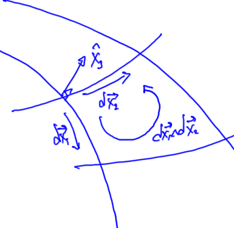
Following the arguments used in [7] for Stokes theorem in three dimensions, we first evaluate the loop integral along the differential element of the surface at the point \mathbf{x}(u_0, v_0) evaluated over the range (du, dv), as shown in the infinitesimal loop of fig. 1.1.

Fig 1.1. Infinitesimal loop integral

Over the infinitesimal area, the loop integral decomposes into

\begin{aligned}\mathop{\rlap{\ensuremath{\mkern3.5mu\circlearrowright}}\int} \mathbf{f} \cdot d\mathbf{l}=\int \mathbf{f} \cdot d\mathbf{x}_1+\int \mathbf{f} \cdot d\mathbf{x}_2+\int \mathbf{f} \cdot d\mathbf{x}_3+\int \mathbf{f} \cdot d\mathbf{x}_4,\end{aligned} \hspace{\stretch{1}}(1.20)

where the differentials along the curve are

\begin{aligned}\begin{aligned}d\mathbf{x}_1 &= {\left.{{ \frac{\partial {\mathbf{x}}}{\partial {u}} }}\right\vert}_{{v = v_0}} du \\ d\mathbf{x}_2 &= {\left.{{ \frac{\partial {\mathbf{x}}}{\partial {v}} }}\right\vert}_{{u = u_0 + du}} dv \\ d\mathbf{x}_3 &= -{\left.{{ \frac{\partial {\mathbf{x}}}{\partial {u}} }}\right\vert}_{{v = v_0 + dv}} du \\ d\mathbf{x}_4 &= -{\left.{{ \frac{\partial {\mathbf{x}}}{\partial {v}} }}\right\vert}_{{u = u_0}} dv.\end{aligned}\end{aligned} \hspace{\stretch{1}}(1.21)

It is assumed that the parameterization change (du, dv) is small enough that this loop integral can be considered planar (regardless of the dimension of the vector space). Making use of the fact that \mathbf{x}^\perp \cdot \mathbf{x}_\alpha = 0 for \alpha \in \left\{ {u,v} \right\}, the loop integral is

\begin{aligned}\mathop{\rlap{\ensuremath{\mkern3.5mu\circlearrowright}}\int} \mathbf{f} \cdot d\mathbf{l}=\int\left( {f_u \mathbf{x}^u + f_v \mathbf{x}^v + f_\perp \mathbf{x}^\perp} \right)\cdot\Bigl(\mathbf{x}_u(u, v_0) du - \mathbf{x}_u(u, v_0 + dv) du+\mathbf{x}_v(u_0 + du, v) dv - \mathbf{x}_v(u_0, v) dv\Bigr)=\int f_u(u, v_0) du - f_u(u, v_0 + dv) du+f_v(u_0 + du, v) dv - f_v(u_0, v) dv\end{aligned} \hspace{\stretch{1}}(1.22)

With the distances being infinitesimal, these differences can be rewritten as partial differentials

\begin{aligned}\mathop{\rlap{\ensuremath{\mkern3.5mu\circlearrowright}}\int} \mathbf{f} \cdot d\mathbf{l}=\iint \left( {-\frac{\partial {f_u}}{\partial {v}}+\frac{\partial {f_v}}{\partial {u}}} \right)du dv.\end{aligned} \hspace{\stretch{1}}(1.23)

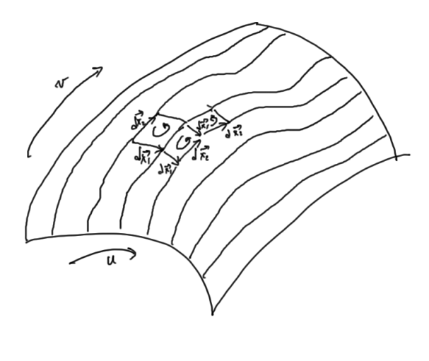
We can now sum over a larger area as in fig. 1.2

Fig 1.2. Sum of infinitesimal loops

All the opposing oriented loop elements cancel, so the integral around the complete boundary of the surface \mathbf{x}(u, v) is given by the u,v area integral of the partials difference.

We will see that Green’s theorem is a special case of the Curl (Stokes) theorem. This observation will also provide a geometric interpretation of the right hand side area integral of thm. 2, and allow for a coordinate free representation.

Special case:

An important special case of Green’s theorem is for a Euclidean two dimensional space where the vector function is

\begin{aligned}\mathbf{f} = P \mathbf{e}_1 + Q \mathbf{e}_2.\end{aligned} \hspace{\stretch{1}}(1.24)

Here Green’s theorem takes the form

\begin{aligned}\mathop{\rlap{\ensuremath{\mkern3.5mu\circlearrowright}}\int} P dx + Q dy=\iint \left( {\frac{\partial {Q}}{\partial {x}}-\frac{\partial {P}}{\partial {y}}} \right)dx dy.\end{aligned} \hspace{\stretch{1}}(1.0.25)

Curl theorem, two volume vector field

Having examined the right hand side of thm. 1 for the very simplest geometric object \mathbf{f}, let’s look at the right hand side, the area integral in more detail. We restrict our attention for now to vectors \mathbf{f} still defined by eq. 1.19.

First we need to assign a meaning to d^2 \mathbf{x}. By this, we mean the wedge products of the two differential elements. With

\begin{aligned}d\mathbf{x}_i = du^i \frac{\partial {\mathbf{x}}}{\partial {u^i}} = du^i \mathbf{x}_i,\end{aligned} \hspace{\stretch{1}}(1.26)

that area element is

\begin{aligned}d^2 \mathbf{x}= d\mathbf{x}_1 \wedge d\mathbf{x}_2= du^1 du^2 \mathbf{x}_1 \wedge \mathbf{x}_2.\end{aligned} \hspace{\stretch{1}}(1.0.27)

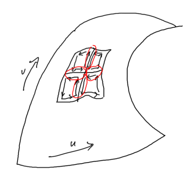
This is the oriented area element that lies in the tangent plane at the point of evaluation, and has the magnitude of the area of that segment of the surface, as depicted in fig. 1.3.

Fig 1.3. Oriented area element tiling of a surface

Observe that we have no requirement to introduce a normal to the surface to describe the direction of the plane. The wedge product provides the information about the orientation of the place in the space, even when the vector space that our vector lies in has dimension greater than three.

Proceeding with the expansion of the dot product of the area element with the curl, using eq. 1.0.6, eq. 1.0.7, and eq. 1.0.8, and a scalar selection operation, we have

\begin{aligned}d^2 \mathbf{x} \cdot \left( { \boldsymbol{\partial} \wedge \mathbf{f} } \right) &= \left\langle{{d^2 \mathbf{x} \left( { \boldsymbol{\partial} \wedge \mathbf{f} } \right)}}\right\rangle \\ &= \left\langle{{d^2 \mathbf{x}\frac{1}{2}\left( { \stackrel{ \rightarrow }{\boldsymbol{\partial}} \mathbf{f} - \mathbf{f} \stackrel{ \leftarrow }{\boldsymbol{\partial}} } \right)}}\right\rangle \\ &= \frac{1}{2}\left\langle{{d^2 \mathbf{x} \left( { \mathbf{x}^i \left( { \partial_i \mathbf{f}} \right) - \left( {\partial_i \mathbf{f}} \right) \mathbf{x}^i } \right)}}\right\rangle \\ &= \frac{1}{2}\left\langle{{\left( { \partial_i \mathbf{f} } \right) d^2 \mathbf{x} \mathbf{x}^i - \left( { \partial_i \mathbf{f} } \right) \mathbf{x}^i d^2 \mathbf{x}}}\right\rangle \\ &= \left\langle{{\left( { \partial_i \mathbf{f} } \right) \left( { d^2 \mathbf{x} \cdot \mathbf{x}^i } \right)}}\right\rangle \\ &= \partial_i \mathbf{f} \cdot\left( { d^2 \mathbf{x} \cdot \mathbf{x}^i } \right).\end{aligned} \hspace{\stretch{1}}(1.28)

Let’s proceed to expand the inner dot product

\begin{aligned}d^2 \mathbf{x} \cdot \mathbf{x}^i &= du^1 du^2\left( { \mathbf{x}_1 \wedge \mathbf{x}_2 } \right) \cdot \mathbf{x}^i \\ &= du^1 du^2\left( {\mathbf{x}_2 \cdot \mathbf{x}^i \mathbf{x}_1-\mathbf{x}_1 \cdot \mathbf{x}^i \mathbf{x}_2} \right) \\ &= du^1 du^2\left( {{\delta_2}^i \mathbf{x}_1-{\delta_1}^i \mathbf{x}_2} \right).\end{aligned} \hspace{\stretch{1}}(1.29)

The complete curl term is thus

\begin{aligned}d^2 \mathbf{x} \cdot \left( { \boldsymbol{\partial} \wedge \mathbf{f} } \right)=du^1 du^2\left( {\frac{\partial {\mathbf{f}}}{\partial {u^2}} \cdot \mathbf{x}_1-\frac{\partial {\mathbf{f}}}{\partial {u^1}} \cdot \mathbf{x}_2} \right)\end{aligned} \hspace{\stretch{1}}(1.30)

This almost has the form of eq. 1.23, although that is not immediately obvious. Working backwards, using the shorthand u = u^1, v = u^2, we can show that this coordinate representation can be eliminated

\begin{aligned}-du dv\left( {\frac{\partial {f_v}}{\partial {u}} -\frac{\partial {f_u}}{\partial {v}}} \right) &= du dv\left( {\frac{\partial {}}{\partial {v}}\left( {\mathbf{f} \cdot \mathbf{x}_u} \right)-\frac{\partial {}}{\partial {u}}\left( {\mathbf{f} \cdot \mathbf{x}_v} \right)} \right) \\ &= du dv\left( {\frac{\partial {\mathbf{f}}}{\partial {v}} \cdot \mathbf{x}_u-\frac{\partial {\mathbf{f}}}{\partial {u}} \cdot \mathbf{x}_v+\mathbf{f} \cdot \left( {\frac{\partial {\mathbf{x}_u}}{\partial {v}}-\frac{\partial {\mathbf{x}_v}}{\partial {u}}} \right)} \right) \\ &= du dv \left( {\frac{\partial {\mathbf{f}}}{\partial {v}} \cdot \mathbf{x}_u-\frac{\partial {\mathbf{f}}}{\partial {u}} \cdot \mathbf{x}_v+\mathbf{f} \cdot \left( {\frac{\partial^2 \mathbf{x}}{\partial v \partial u}-\frac{\partial^2 \mathbf{x}}{\partial u \partial v}} \right)} \right) \\ &= du dv \left( {\frac{\partial {\mathbf{f}}}{\partial {v}} \cdot \mathbf{x}_u-\frac{\partial {\mathbf{f}}}{\partial {u}} \cdot \mathbf{x}_v} \right) \\ &= d^2 \mathbf{x} \cdot \left( { \boldsymbol{\partial} \wedge \mathbf{f} } \right).\end{aligned} \hspace{\stretch{1}}(1.31)

This relates the two parameter surface integral of the curl to the loop integral over its boundary

\begin{aligned}\int d^2 \mathbf{x} \cdot (\boldsymbol{\partial} \wedge \mathbf{f}) = \mathop{\rlap{\ensuremath{\mkern3.5mu\circlearrowleft}}\int} \mathbf{f} \cdot d\mathbf{l}.\end{aligned} \hspace{\stretch{1}}(1.0.32)

This is the very simplest special case of Stokes theorem. When written in the general form of Stokes thm. 1

\begin{aligned}\int_A d^2 \mathbf{x} \cdot \left( { \boldsymbol{\partial} \wedge \mathbf{f}} \right)=\int_{\partial A} d^1 \mathbf{x} \cdot \mathbf{f}=\int_{\partial A} \left( { d\mathbf{x}_1 - d\mathbf{x}_2 } \right) \cdot \mathbf{f},\end{aligned} \hspace{\stretch{1}}(1.0.33)

we must remember (the \partial A is to remind us of this) that it is implied that both the vector \mathbf{f} and the differential elements are evaluated on the boundaries of the integration ranges respectively. A more exact statement is

\begin{aligned}\int_{\partial A} d^1 \mathbf{x} \cdot \mathbf{f}=\int {\left.{{\mathbf{f} \cdot d\mathbf{x}_1}}\right\vert}_{{\Delta u^2}}-{\left.{{\mathbf{f} \cdot d\mathbf{x}_2}}\right\vert}_{{\Delta u^1}}=\int {\left.{{f_1}}\right\vert}_{{\Delta u^2}} du^1-{\left.{{f_2}}\right\vert}_{{\Delta u^1}} du^2.\end{aligned} \hspace{\stretch{1}}(1.0.34)

Expanded out in full this is

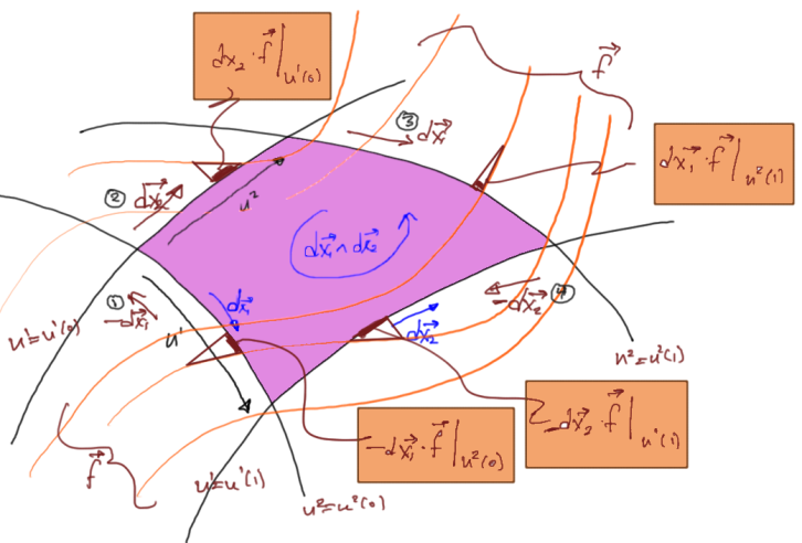
\begin{aligned}\int {\left.{{\mathbf{f} \cdot d\mathbf{x}_1}}\right\vert}_{{u^2(1)}}-{\left.{{\mathbf{f} \cdot d\mathbf{x}_1}}\right\vert}_{{u^2(0)}}+{\left.{{\mathbf{f} \cdot d\mathbf{x}_2}}\right\vert}_{{u^1(0)}}-{\left.{{\mathbf{f} \cdot d\mathbf{x}_2}}\right\vert}_{{u^1(1)}},\end{aligned} \hspace{\stretch{1}}(1.0.35)

which can be cross checked against fig. 1.4 to demonstrate that this specifies a clockwise orientation. For the surface with oriented area d\mathbf{x}_1 \wedge d\mathbf{x}_2, the clockwise loop is designated with line elements (1)-(4), we see that the contributions around this loop (in boxes) match eq. 1.0.35.

Fig 1.4. Clockwise loop

Example: Green’s theorem, a 2D Cartesian parameterization for a Euclidean space

For a Cartesian 2D Euclidean parameterization of a vector field and the integration space, Stokes theorem should be equivalent to Green’s theorem eq. 1.0.25. Let’s expand both sides of eq. 1.0.32 independently to verify equality. The parameterization is

\begin{aligned}\mathbf{x}(x, y) = x \mathbf{e}_1 + y \mathbf{e}_2.\end{aligned} \hspace{\stretch{1}}(1.36)

Here the dual basis is the basis, and the projection onto the tangent space is just the gradient

\begin{aligned}\boldsymbol{\partial} = \boldsymbol{\nabla}= \mathbf{e}_1 \frac{\partial {}}{\partial {x}}+ \mathbf{e}_2 \frac{\partial {}}{\partial {y}}.\end{aligned} \hspace{\stretch{1}}(1.0.37)

The volume element is an area weighted pseudoscalar for the space

\begin{aligned}d^2 \mathbf{x} = dx dy \frac{\partial {\mathbf{x}}}{\partial {x}} \wedge \frac{\partial {\mathbf{x}}}{\partial {y}} = dx dy \mathbf{e}_1 \mathbf{e}_2,\end{aligned} \hspace{\stretch{1}}(1.0.38)

and the curl of a vector \mathbf{f} = f_1 \mathbf{e}_1 + f_2 \mathbf{e}_2 is

\begin{aligned}\boldsymbol{\partial} \wedge \mathbf{f}=\left( {\mathbf{e}_1 \frac{\partial {}}{\partial {x}}+ \mathbf{e}_2 \frac{\partial {}}{\partial {y}}} \right) \wedge\left( {f_1 \mathbf{e}_1 + f_2 \mathbf{e}_2} \right)=\mathbf{e}_1 \mathbf{e}_2\left( {\frac{\partial {f_2}}{\partial {x}}-\frac{\partial {f_1}}{\partial {y}}} \right).\end{aligned} \hspace{\stretch{1}}(1.0.38)

So, the LHS of Stokes theorem takes the coordinate form

\begin{aligned}\int d^2 \mathbf{x} \cdot (\boldsymbol{\partial} \wedge \mathbf{f}) =\iint dx dy\underbrace{\left\langle{{\mathbf{e}_1 \mathbf{e}_2 \mathbf{e}_1 \mathbf{e}_2}}\right\rangle}_{=-1}\left( {\frac{\partial {f_2}}{\partial {x}}-\frac{\partial {f_1}}{\partial {y}}} \right).\end{aligned} \hspace{\stretch{1}}(1.0.38)

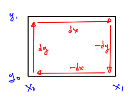
For the RHS, following fig. 1.5, we have

\begin{aligned}\mathop{\rlap{\ensuremath{\mkern3.5mu\circlearrowleft}}\int} \mathbf{f} \cdot d\mathbf{x}=f_2(x_0, y) dy+f_1(x, y_1) dx-f_2(x_1, y) dy-f_1(x, y_0) dx=\int dx \left( {f_1(x, y_1)-f_1(x, y_0)} \right)-\int dy \left( {f_2(x_1, y)-f_2(x_0, y)} \right).\end{aligned} \hspace{\stretch{1}}(1.0.38)

As expected, we can also obtain this by integrating eq. 1.0.38.

Fig 1.5. Euclidean 2D loop

Example: Cylindrical parameterization

Let’s now consider a cylindrical parameterization of a 4D space with Euclidean metric ++++ or Minkowski metric +++-. For such a space let’s do a brute force expansion of both sides of Stokes theorem to gain some confidence that all is well.

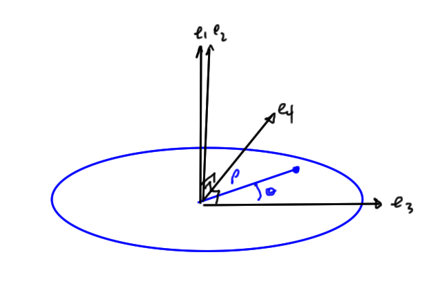
With \kappa = \mathbf{e}_3 \mathbf{e}_4, such a space is conveniently parameterized as illustrated in fig. 1.6 as

\begin{aligned}\mathbf{x}(\rho, \theta, h) = x \mathbf{e}_1 + y \mathbf{e}_2 + \rho \mathbf{e}_3 e^{\kappa \theta}.\end{aligned} \hspace{\stretch{1}}(1.42)

Fig 1.6. Cylindrical polar parameterization

Note that the Euclidean case where \left( {\mathbf{e}_4} \right)^2 = 1 rejection of the non-axial components of \mathbf{x} expands to

\begin{aligned}\left( { \left( { \mathbf{x} \wedge \mathbf{e}_1 \wedge \mathbf{e}_2} \right) \cdot \mathbf{e}^2 } \right) \cdot \mathbf{e}^1 =\rho \left( { \mathbf{e}_3 \cos\theta + \mathbf{e}_4 \sin \theta } \right),\end{aligned} \hspace{\stretch{1}}(1.43)

whereas for the Minkowski case where \left( {\mathbf{e}_4} \right)^2 = -1 we have a hyperbolic expansion

\begin{aligned}\left( { \left( { \mathbf{x} \wedge \mathbf{e}_1 \wedge \mathbf{e}_2} \right) \cdot \mathbf{e}^2 } \right) \cdot \mathbf{e}^1 =\rho \left( { \mathbf{e}_3 \cosh\theta + \mathbf{e}_4 \sinh \theta } \right).\end{aligned} \hspace{\stretch{1}}(1.44)

Within such a space consider the surface along x = c, y = d, for which the vectors are parameterized by

\begin{aligned}\mathbf{x}(\rho, \theta) = c \mathbf{e}_1 + d \mathbf{e}_2 + \rho \mathbf{e}_3 e^{\kappa \theta}.\end{aligned} \hspace{\stretch{1}}(1.45)

The tangent space unit vectors are

\begin{aligned}\mathbf{x}_\rho= \frac{\partial {\mathbf{x}}}{\partial {\rho}} = \mathbf{e}_3 e^{\kappa \theta},\end{aligned} \hspace{\stretch{1}}(1.46)

and

\begin{aligned}\mathbf{x}_\theta &= \frac{\partial {\mathbf{x}}}{\partial {\theta}} \\ &= \rho \mathbf{e}_3 \mathbf{e}_3 \mathbf{e}_4 e^{\kappa \theta} \\ &= \rho \mathbf{e}_4 e^{\kappa \theta}.\end{aligned} \hspace{\stretch{1}}(1.47)

Observe that both of these vectors have their origin at the point of evaluation, and aren’t relative to the absolute origin used to parameterize the complete space.

We wish to compute the volume element for the tangent plane. Noting that \mathbf{e}_3 and \mathbf{e}_4 both anticommute with \kappa we have for \mathbf{a} \in \text{span} \left\{ {\mathbf{e}_3, \mathbf{e}_4} \right\}

\begin{aligned}\mathbf{a} e^{\kappa \theta} = e^{-\kappa \theta} \mathbf{a},\end{aligned} \hspace{\stretch{1}}(1.48)

so

\begin{aligned}\mathbf{x}_\theta \wedge \mathbf{x}_\rho &= {\left\langle{{\mathbf{e}_3 e^{\kappa \theta} \rho \mathbf{e}_4 e^{\kappa \theta}}}\right\rangle}_{2} \\ &= \rho {\left\langle{{\mathbf{e}_3 e^{\kappa \theta} e^{-\kappa \theta} \mathbf{e}_4}}\right\rangle}_{2} \\ &= \rho \mathbf{e}_3 \mathbf{e}_4.\end{aligned} \hspace{\stretch{1}}(1.49)

The tangent space volume element is thus

\begin{aligned}d^2 \mathbf{x} = \rho d\rho d\theta \mathbf{e}_3 \mathbf{e}_4.\end{aligned} \hspace{\stretch{1}}(1.50)

With the tangent plane vectors both perpendicular we don’t need the general lemma 6 to compute the reciprocal basis, but can do so by inspection

\begin{aligned}\mathbf{x}^\rho = e^{-\kappa \theta} \mathbf{e}^3,\end{aligned} \hspace{\stretch{1}}(1.0.51)

and

\begin{aligned}\mathbf{x}^\theta = e^{-\kappa \theta} \mathbf{e}^4 \frac{1}{{\rho}}.\end{aligned} \hspace{\stretch{1}}(1.0.52)

Observe that the latter depends on the metric signature.

The vector derivative, the projection of the gradient on the tangent space, is

\begin{aligned}\boldsymbol{\partial} &= \mathbf{x}^\rho \frac{\partial {}}{\partial {\rho}}+\mathbf{x}^\theta \frac{\partial {}}{\partial {\theta}} \\ &= e^{-\kappa \theta} \left( {\mathbf{e}^3 \partial_\rho + \frac{\mathbf{e}^4}{\rho} \partial_\theta } \right).\end{aligned} \hspace{\stretch{1}}(1.0.52)

From this we see that acting with the vector derivative on a scalar radial only dependent function f(\rho) is a vector function that has a radial direction, whereas the action of the vector derivative on an azimuthal only dependent function g(\theta) is a vector function that has only an azimuthal direction. The interpretation of the geometric product action of the vector derivative on a vector function is not as simple since the product will be a multivector.

Expanding the curl in coordinates is messier, but yields in the end when tackled with sufficient care

\begin{aligned}\boldsymbol{\partial} \wedge \mathbf{f} &= {\left\langle{{e^{-\kappa \theta}\left( { e^3 \partial_\rho + \frac{e^4}{\rho} \partial_\theta} \right)\left( { \not{{e_1 x}} + \not{{e_2 y}} + e_3 e^{\kappa \theta } f_\rho + \frac{e^4}{\rho} e^{\kappa \theta } f_\theta} \right)}}\right\rangle}_{2} \\ &= \not{{{\left\langle{{e^{-\kappa \theta} e^3 \partial_\rho \left( { e_3 e^{\kappa \theta } f_\rho} \right)}}\right\rangle}_{2}}}+{\left\langle{{\not{{e^{-\kappa \theta}}} e^3 \partial_\rho \left( { \frac{e^4}{\rho} \not{{e^{\kappa \theta }}} f_\theta} \right)}}\right\rangle}_{2}+{\left\langle{{e^{-\kappa \theta}\frac{e^4}{\rho} \partial_\theta\left( { e_3 e^{\kappa \theta } f_\rho} \right)}}\right\rangle}_{2}+{\left\langle{{e^{-\kappa \theta}\frac{e^4}{\rho} \partial_\theta\left( { \frac{e^4}{\rho} e^{\kappa \theta } f_\theta} \right)}}\right\rangle}_{2} \\ &= \mathbf{e}^3 \mathbf{e}^4 \left( {-\frac{f_\theta}{\rho^2} + \frac{1}{{\rho}} \partial_\rho f_\theta- \frac{1}{{\rho}} \partial_\theta f_\rho} \right)+ \frac{1}{{\rho^2}}{\left\langle{{e^{-\kappa \theta} \left( {\mathbf{e}^4} \right)^2\left( {\mathbf{e}_3 \mathbf{e}_4 f_\theta+ \not{{\partial_\theta f_\theta}}} \right)e^{\kappa \theta}}}\right\rangle}_{2} \\ &= \mathbf{e}^3 \mathbf{e}^4 \left( {-\frac{f_\theta}{\rho^2} + \frac{1}{{\rho}} \partial_\rho f_\theta- \frac{1}{{\rho}} \partial_\theta f_\rho} \right)+ \frac{1}{{\rho^2}}{\left\langle{{\not{{e^{-\kappa \theta} }}\mathbf{e}_3 \mathbf{e}^4 f_\theta\not{{e^{\kappa \theta}}}}}\right\rangle}_{2} \\ &= \frac{\mathbf{e}^3 \mathbf{e}^4 }{\rho}\left( {\partial_\rho f_\theta- \partial_\theta f_\rho} \right).\end{aligned} \hspace{\stretch{1}}(1.0.52)

After all this reduction, we can now state in coordinates the LHS of Stokes theorem explicitly

\begin{aligned}\int d^2 \mathbf{x} \cdot \left( { \boldsymbol{\partial} \wedge \mathbf{f} } \right) &= \int \rho d\rho d\theta \left\langle{{\mathbf{e}_3 \mathbf{e}_4 \mathbf{e}^3 \mathbf{e}^4 }}\right\rangle\frac{1}{{\rho}}\left( {\partial_\rho f_\theta- \partial_\theta f_\rho} \right) \\ &= \int d\rho d\theta\left( {\partial_\theta f_\rho-\partial_\rho f_\theta} \right) \\ &= \int d\rho {\left.{{f_\rho}}\right\vert}_{{\Delta \theta}}- \int d\theta{\left.{{f_\theta}}\right\vert}_{{\Delta \rho}}.\end{aligned} \hspace{\stretch{1}}(1.0.52)

Now compare this to the direct evaluation of the loop integral portion of Stokes theorem. Expressing this using eq. 1.0.34, we have the same result

\begin{aligned}\int d^2 \mathbf{x} \cdot \left( { \boldsymbol{\partial} \wedge \mathbf{f} } \right)=\int {\left.{{f_\rho}}\right\vert}_{{\Delta \theta}} d\rho-{\left.{{f_\theta}}\right\vert}_{{\Delta \rho}} d\theta\end{aligned} \hspace{\stretch{1}}(1.0.56)

This example highlights some of the power of Stokes theorem, since the reduction of the volume element differential form was seen to be quite a chore (and easy to make mistakes doing.)

Example: Composition of boost and rotation

Working in a \bigwedge^{1,3} space with basis \left\{ {\gamma_0, \gamma_1, \gamma_2, \gamma_3} \right\} where \left( {\gamma_0} \right)^2 = 1 and \left( {\gamma_k} \right)^2 = -1, k \in \left\{ {1,2,3} \right\}, an active composition of boost and rotation has the form

\begin{aligned}\begin{aligned}\mathbf{x}' &= e^{i\alpha/2} \mathbf{x}_0 e^{-i\alpha/2} \\ \mathbf{x}'' &= e^{-j\theta/2} \mathbf{x}' e^{j\theta/2}\end{aligned},\end{aligned} \hspace{\stretch{1}}(1.0.57)

where i is a bivector of a timelike unit vector and perpendicular spacelike unit vector, and j is a bivector of two perpendicular spacelike unit vectors. For example, i = \gamma_0 \gamma_1 and j = \gamma_1 \gamma_2. For such i,j the respective Lorentz transformation matrices are

\begin{aligned}{\begin{bmatrix}x^0 \\ x^1 \\ x^2 \\ x^3 \end{bmatrix}}'=\begin{bmatrix}\cosh\alpha & -\sinh\alpha & 0 & 0 \\ -\sinh\alpha & \cosh\alpha & 0 & 0 \\ 0 & 0 & 1 & 0 \\ 0 & 0 & 0 & 1 \end{bmatrix}\begin{bmatrix}x^0 \\ x^1 \\ x^2 \\ x^3 \end{bmatrix},\end{aligned} \hspace{\stretch{1}}(1.0.58)

and

\begin{aligned}{\begin{bmatrix}x^0 \\ x^1 \\ x^2 \\ x^3 \end{bmatrix}}''=\begin{bmatrix}1 & 0 & 0 & 0 \\ 0 & \cos\theta & \sin\theta & 0 \\ 0 & -\sin\theta & \cos\theta & 0 \\ 0 & 0 & 0 & 1 \end{bmatrix}{\begin{bmatrix}x^0 \\ x^1 \\ x^2 \\ x^3 \end{bmatrix}}'.\end{aligned} \hspace{\stretch{1}}(1.0.59)

Let’s calculate the tangent space vectors for this parameterization, assuming that the particle is at an initial spacetime position of \mathbf{x}_0. That is

\begin{aligned}\mathbf{x} = e^{-j\theta/2} e^{i\alpha/2} \mathbf{x}_0e^{-i\alpha/2} e^{j\theta/2}.\end{aligned} \hspace{\stretch{1}}(1.0.60)

To calculate the tangent space vectors for this subspace we note that

\begin{aligned}\frac{\partial {\mathbf{x}'}}{\partial {\alpha}} = \frac{i}{2} \mathbf{x}_0 - \mathbf{x}_0 \frac{i}{2} = i \cdot \mathbf{x}_0,\end{aligned} \hspace{\stretch{1}}(1.0.61)

and

\begin{aligned}\frac{\partial {\mathbf{x}''}}{\partial {\theta}} = -\frac{j}{2} \mathbf{x}' + \mathbf{x}' \frac{j}{2} = \mathbf{x}' \cdot j.\end{aligned} \hspace{\stretch{1}}(1.0.62)

The tangent space vectors are therefore

\begin{aligned}\begin{aligned}\mathbf{x}_\alpha &= e^{-j\theta/2} \left( { i \cdot \mathbf{x}_0 } \right)e^{j\theta/2} \\ \mathbf{x}_\theta &= \left( {e^{i\alpha/2} \mathbf{x}_0e^{-i\alpha/2} } \right) \cdot j.\end{aligned}\end{aligned} \hspace{\stretch{1}}(1.0.63)

Continuing a specific example where i = \gamma_0\gamma_1, j = \gamma_1 \gamma_2 let’s also pick \mathbf{x}_0 = \gamma_0, the spacetime position of a particle at the origin of a frame at that frame’s c t = 1. The tangent space vectors for the subspace parameterized by this transformation and this initial position is then reduced to

\begin{aligned}\mathbf{x}_\alpha = -\gamma_1 e^{j \theta} = \gamma_1 \sin\theta + \gamma_2 \cos\theta,\end{aligned} \hspace{\stretch{1}}(1.0.63)

and

\begin{aligned}\mathbf{x}_\theta &= \left( { \gamma_0 e^{-i \alpha} } \right) \cdot j \\ &= \left( { \gamma_0\left( { \cosh\alpha - \gamma_0 \gamma_1 \sinh\alpha } \right)} \right) \cdot \left( { \gamma_1 \gamma_2} \right) \\ &= {\left\langle{{ \left( { \gamma_0 \cosh\alpha - \gamma_1 \sinh\alpha } \right) \gamma_1 \gamma_2 }}\right\rangle}_{1} \\ &= \gamma_2 \sinh\alpha.\end{aligned} \hspace{\stretch{1}}(1.0.63)

By inspection the dual basis for this parameterization is

\begin{aligned}\begin{aligned}\mathbf{x}^\alpha &= \gamma_1 e^{j \theta} \\ \mathbf{x}^\theta &= \frac{\gamma^2}{\sinh\alpha} \end{aligned}\end{aligned} \hspace{\stretch{1}}(1.0.66)

So, Stokes theorem, applied to a spacetime vector \mathbf{f}, for this subspace is

\begin{aligned}\int d\alpha d\theta \sinh\alpha \sin\theta \left( { \gamma_1 \gamma_2 } \right) \cdot \left( {\left( {\gamma_1 e^{j \theta} \partial_\alpha + \frac{\gamma^2}{\sinh\alpha} \partial_\theta} \right)\wedge \mathbf{f}} \right)=\int d\alpha {\left.{{\mathbf{f} \cdot \Bigl( {\gamma^1 e^{j \theta}} \Bigr)}}\right\vert}_{{\theta_0}}^{{\theta_1}}-\int d\theta {\left.{{\mathbf{f} \cdot \Bigl( { \gamma_2 \sinh\alpha } \Bigr)}}\right\vert}_{{\alpha_0}}^{{\alpha_1}}.\end{aligned} \hspace{\stretch{1}}(1.0.67)

Since the point is to avoid the curl integral, we did not actually have to state it explicitly, nor was there any actual need to calculate the dual basis.

Example: Dual representation in three dimensions

It’s clear that there is a projective nature to the differential form d^2 \mathbf{x} \cdot \left( {\boldsymbol{\partial} \wedge \mathbf{f}} \right). This projective nature allows us, in three dimensions, to re-express Stokes theorem using the gradient instead of the vector derivative, and to utilize the cross product and a normal direction to the plane.

When we parameterize a normal direction to the tangent space, so that for a 2D tangent space spanned by curvilinear coordinates \mathbf{x}_1 and \mathbf{x}_2 the vector \mathbf{x}^3 is normal to both, we can write our vector as

\begin{aligned}\mathbf{f} = f_1 \mathbf{x}^1 + f_2 \mathbf{x}^2 + f_3 \mathbf{x}^3,\end{aligned} \hspace{\stretch{1}}(1.0.68)

and express the orientation of the tangent space area element in terms of a pseudoscalar that includes this normal direction

\begin{aligned}\mathbf{x}_1 \wedge \mathbf{x}_2 =\mathbf{x}^3 \cdot \left( { \mathbf{x}_1 \wedge \mathbf{x}_2 \wedge \mathbf{x}_3 } \right) =\mathbf{x}^3 \left( { \mathbf{x}_1 \wedge \mathbf{x}_2 \wedge \mathbf{x}_3 } \right).\end{aligned} \hspace{\stretch{1}}(1.0.69)

Inserting this into an expansion of the curl form we have

\begin{aligned}d^2 \mathbf{x} \cdot \left( { \boldsymbol{\partial} \wedge \mathbf{f} } \right) &= du^1 du^2 \left\langle{{\mathbf{x}^3 \left( { \mathbf{x}_1 \wedge \mathbf{x}_2 \wedge \mathbf{x}_3 } \right)\left( {\left( {\sum_{i=1,2} x^i \partial_i} \right)\wedge\mathbf{f}} \right)}}\right\rangle \\ &= du^1 du^2 \mathbf{x}^3 \cdot \left( {\left( { \mathbf{x}_1 \wedge \mathbf{x}_2 \wedge \mathbf{x}_3 } \right)\cdot \left( {\boldsymbol{\nabla} \wedge \mathbf{f}} \right)-\left( { \mathbf{x}_1 \wedge \mathbf{x}_2 \wedge \mathbf{x}_3 } \right)\cdot \left( {\mathbf{x}^3 \partial_3 \wedge \mathbf{f}} \right)} \right).\end{aligned} \hspace{\stretch{1}}(1.0.69)

Observe that this last term, the contribution of the component of the gradient perpendicular to the tangent space, has no \mathbf{x}_3 components

\begin{aligned}\left( { \mathbf{x}_1 \wedge \mathbf{x}_2 \wedge \mathbf{x}_3 } \right)\cdot \left( {\mathbf{x}^3 \partial_3 \wedge \mathbf{f}} \right) &= \left( { \mathbf{x}_1 \wedge \mathbf{x}_2 \wedge \mathbf{x}_3 } \right)\cdot \left( {\mathbf{x}^3 \wedge \partial_3 \mathbf{f}} \right) \\ &= \left( { \left( { \mathbf{x}_1 \wedge \mathbf{x}_2 \wedge \mathbf{x}_3 } \right) \cdot \mathbf{x}^3} \right)\cdot \partial_3 \mathbf{f} \\ &= \left( { \mathbf{x}_1 \wedge \mathbf{x}_2 } \right) \cdot \partial_3 \mathbf{f} \\ &= \mathbf{x}_1 \left( { \mathbf{x}_2 \cdot \partial_3 \mathbf{f} } \right)-\mathbf{x}_2 \left( { \mathbf{x}_1 \cdot \partial_3 \mathbf{f} } \right),\end{aligned} \hspace{\stretch{1}}(1.0.69)

leaving

\begin{aligned}d^2 \mathbf{x} \cdot \left( { \boldsymbol{\partial} \wedge \mathbf{f} } \right)=du^1 du^2 \mathbf{x}^3 \cdot \left( {\left( { \mathbf{x}_1 \wedge \mathbf{x}_2 \wedge \mathbf{x}_3 } \right) \cdot \left( { \boldsymbol{\nabla} \wedge \mathbf{f}} \right)} \right).\end{aligned} \hspace{\stretch{1}}(1.0.69)

Now scale the normal vector and its dual to have unit norm as follows

\begin{aligned}\begin{aligned}\mathbf{x}^3 &= \alpha \hat{\mathbf{x}}^3 \\ \mathbf{x}_3 &= \frac{1}{{\alpha}} \hat{\mathbf{x}}_3,\end{aligned}\end{aligned} \hspace{\stretch{1}}(1.0.73)

so that for \beta > 0, the volume element can be

\begin{aligned}\mathbf{x}_1 \wedge \mathbf{x}_2 \wedge \hat{\mathbf{x}}_3 = \beta I.\end{aligned} \hspace{\stretch{1}}(1.0.73)

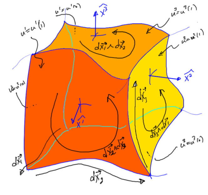
This scaling choice is illustrated in fig. 1.7, and represents the “outwards” normal. With such a scaling choice we have

Fig 1.7. Outwards normal

\begin{aligned}\beta du^1 du^2 = dA,\end{aligned} \hspace{\stretch{1}}(1.75)

and almost have the desired cross product representation

\begin{aligned}d^2 \mathbf{x} \cdot \left( { \boldsymbol{\partial} \wedge \mathbf{f} } \right)=dA \hat{\mathbf{x}}^3 \cdot \left( { I \cdot \left( {\boldsymbol{\nabla} \wedge \mathbf{f}} \right) } \right)=dA \hat{\mathbf{x}}^3 \cdot \left( { I \left( {\boldsymbol{\nabla} \wedge \mathbf{f}} \right) } \right).\end{aligned} \hspace{\stretch{1}}(1.76)

With the duality identity \mathbf{a} \wedge \mathbf{b} = I \left( {\mathbf{a} \times \mathbf{b}} \right), we have the traditional 3D representation of Stokes theorem

\begin{aligned}\int d^2 \mathbf{x} \cdot \left( { \boldsymbol{\partial} \wedge \mathbf{f} } \right)=-\int dA \hat{\mathbf{x}}^3 \cdot \left( {\boldsymbol{\nabla} \times \mathbf{f}} \right) = \mathop{\rlap{\ensuremath{\mkern3.5mu\circlearrowleft}}\int} \mathbf{f} \cdot d\mathbf{l}.\end{aligned} \hspace{\stretch{1}}(1.0.77)

Note that the orientation of the loop integral in the traditional statement of the 3D Stokes theorem is counterclockwise instead of clockwise, as written here.

Stokes theorem, three variable volume element parameterization

We can restate the identity of thm. 1 in an equivalent dot product form.

\begin{aligned}\int_V \left( { d^k \mathbf{x} \cdot \mathbf{x}^i } \right) \cdot \partial_i F = \int_{\partial V} d^{k-1} \mathbf{x} \cdot F.\end{aligned} \hspace{\stretch{1}}(1.0.78)

Here d^{k-1} \mathbf{x} = \sum_i d^k \mathbf{x} \cdot \mathbf{x}^i, with the implicit assumption that it and the blade F that it is dotted with, are both evaluated at the end points of integration variable u^i that has been integrated against.

We’ve seen one specific example of this above in the expansions of eq. 1.28, and eq. 1.29, however, the equivalent result of eq. 1.0.78, somewhat magically, applies to any degree blade and volume element provided the degree of the blade is less than that of the volume element (i.e. s < k). That magic follows directly from lemma 1.

As an expositional example, consider a three variable volume element parameterization, and a vector blade \mathbf{f}

\begin{aligned}d^3 \mathbf{x} \cdot \left( { \boldsymbol{\partial} \wedge \mathbf{f} } \right) &= \left( { d^3 \mathbf{x} \cdot \mathbf{x}^i } \right) \cdot \partial_i \mathbf{f} \\ &= du^1 du^2 du^3\left( {\left( { \mathbf{x}_1 \wedge \mathbf{x}_2 \wedge \mathbf{x}_3 } \right) \cdot \mathbf{x}^i } \right) \cdot \partial_i \mathbf{f} \\ &= du^1 du^2 du^3\left( {\left( { \mathbf{x}_1 \wedge \mathbf{x}_2 } \right) {\delta_3}^i-\left( { \mathbf{x}_1 \wedge \mathbf{x}_3 } \right) {\delta_2}^i+\left( { \mathbf{x}_2 \wedge \mathbf{x}_3 } \right) {\delta_1}^i} \right) \cdot \partial_i \mathbf{f} \\ &= du^1 du^2 du^3\left( {\left( { \mathbf{x}_1 \wedge \mathbf{x}_2 } \right) \cdot \partial_3 \mathbf{f}-\left( { \mathbf{x}_1 \wedge \mathbf{x}_3 } \right) \cdot \partial_2 \mathbf{f}+\left( { \mathbf{x}_2 \wedge \mathbf{x}_3 } \right) \cdot \partial_1 \mathbf{f}} \right).\end{aligned} \hspace{\stretch{1}}(1.0.78)

It should not be surprising that this has the structure found in the theory of differential forms. Using the differentials for each of the parameterization “directions”, we can write this dot product expansion as

\begin{aligned}d^3 \mathbf{x} \cdot \left( { \boldsymbol{\partial} \wedge \mathbf{f} } \right)=\left( {du^3 \left( { d\mathbf{x}_1 \wedge d\mathbf{x}_2 } \right) \cdot \partial_3 \mathbf{f}-du^2 \left( { d\mathbf{x}_1 \wedge d\mathbf{x}_3 } \right) \cdot \partial_2 \mathbf{f}+du^1 \left( { d\mathbf{x}_2 \wedge d\mathbf{x}_3 } \right) \cdot \partial_1 \mathbf{f}} \right).\end{aligned} \hspace{\stretch{1}}(1.0.78)

Observe that the sign changes with each element of d\mathbf{x}_1 \wedge d\mathbf{x}_2 \wedge d\mathbf{x}_3 that is skipped. In differential forms, the wedge product composition of 1-forms is an abstract quantity. Here the differentials are just vectors, and their wedge product represents an oriented volume element. This interpretation is likely available in the theory of differential forms too, but is arguably less obvious.

Digression

As was the case with the loop integral, we expect that the coordinate representation has a representation that can be expressed as a number of antisymmetric terms. A bit of experimentation shows that such a sum, after dropping the parameter space volume element factor, is

\begin{aligned}\mathbf{x}_1 \left( { -\partial_2 f_3 + \partial_3 f_2 } \right)+\mathbf{x}_2 \left( { -\partial_3 f_1 + \partial_1 f_3 } \right)+\mathbf{x}_3 \left( { -\partial_1 f_2 + \partial_2 f_1 } \right) &= \mathbf{x}_1 \left( { -\partial_2 \mathbf{f} \cdot \mathbf{x}_3 + \partial_3 \mathbf{f} \cdot \mathbf{x}_2 } \right)+\mathbf{x}_2 \left( { -\partial_3 \mathbf{f} \cdot \mathbf{x}_1 + \partial_1 \mathbf{f} \cdot \mathbf{x}_3 } \right)+\mathbf{x}_3 \left( { -\partial_1 \mathbf{f} \cdot \mathbf{x}_2 + \partial_2 \mathbf{f} \cdot \mathbf{x}_1 } \right) \\ &= \left( { \mathbf{x}_1 \partial_3 \mathbf{f} \cdot \mathbf{x}_2 -\mathbf{x}_2 \partial_3 \mathbf{f} \cdot \mathbf{x}_1 } \right)+\left( { \mathbf{x}_3 \partial_2 \mathbf{f} \cdot \mathbf{x}_1 -\mathbf{x}_1 \partial_2 \mathbf{f} \cdot \mathbf{x}_3 } \right)+\left( { \mathbf{x}_2 \partial_1 \mathbf{f} \cdot \mathbf{x}_3 -\mathbf{x}_3 \partial_1 \mathbf{f} \cdot \mathbf{x}_2 } \right) \\ &= \left( { \mathbf{x}_1 \wedge \mathbf{x}_2 } \right) \cdot \partial_3 \mathbf{f}+\left( { \mathbf{x}_3 \wedge \mathbf{x}_1 } \right) \cdot \partial_2 \mathbf{f}+\left( { \mathbf{x}_2 \wedge \mathbf{x}_3 } \right) \cdot \partial_1 \mathbf{f}.\end{aligned} \hspace{\stretch{1}}(1.0.78)

To proceed with the integration, we must again consider an infinitesimal volume element, for which the partial can be evaluated as the difference of the endpoints, with all else held constant. For this three variable parameterization, say, (u,v,w), let’s delimit such an infinitesimal volume element by the parameterization ranges [u_0,u_0 + du], [v_0,v_0 + dv], [w_0,w_0 + dw]. The integral is

\begin{aligned}\begin{aligned}\int_{u = u_0}^{u_0 + du}\int_{v = v_0}^{v_0 + dv}\int_{w = w_0}^{w_0 + dw}d^3 \mathbf{x} \cdot \left( { \boldsymbol{\partial} \wedge \mathbf{f} } \right)&=\int_{u = u_0}^{u_0 + du}du\int_{v = v_0}^{v_0 + dv}dv{\left.{{ \Bigl( { \left( { \mathbf{x}_u \wedge \mathbf{x}_v } \right) \cdot \mathbf{f} } \Bigr) }}\right\vert}_{{w = w_0}}^{{w_0 + dw}} \\ &-\int_{u = u_0}^{u_0 + du}du\int_{w = w_0}^{w_0 + dw}dw{\left.{{\Bigl( { \left( { \mathbf{x}_u \wedge \mathbf{x}_w } \right) \cdot \mathbf{f} } \Bigr) }}\right\vert}_{{v = v_0}}^{{v_0 + dv}} \\ &+\int_{v = v_0}^{v_0 + dv}dv\int_{w = w_0}^{w_0 + dw}dw{\left.{{\Bigl( { \left( { \mathbf{x}_v \wedge \mathbf{x}_w } \right) \cdot \mathbf{f} } \Bigr) }}\right\vert}_{{u = u_0}}^{{u_0 + du}}.\end{aligned}\end{aligned} \hspace{\stretch{1}}(1.0.82)

Extending this over the ranges [u_0,u_0 + \Delta u], [v_0,v_0 + \Delta v], [w_0,w_0 + \Delta w], we have proved Stokes thm. 1 for vectors and a three parameter volume element, provided we have a surface element of the form

\begin{aligned}d^2 \mathbf{x} = {\left. \Bigl( {d\mathbf{x}_u \wedge d\mathbf{x}_v } \Bigr) \right\vert}_{w = w_0}^{w_1}-{\left. \Bigl( {d\mathbf{x}_u \wedge d\mathbf{x}_w } \Bigr) \right\vert}_{v = v_0}^{v_1}+{\left. \Bigl( {d\mathbf{x}_v \wedge \mathbf{x}_w } \Bigr) \right\vert}_{ u = u_0 }^{u_1},\end{aligned} \hspace{\stretch{1}}(1.0.82)

where the evaluation of the dot products with \mathbf{f} are also evaluated at the same points.

Example: Euclidean spherical polar parameterization of 3D subspace

Consider an Euclidean space where a 3D subspace is parameterized using spherical coordinates, as in

\begin{aligned}\mathbf{x}(x, \rho, \theta, \phi) = \mathbf{e}_1 x + \mathbf{e}_4 \rho \exp\left( { \mathbf{e}_4 \mathbf{e}_2 e^{\mathbf{e}_2 \mathbf{e}_3 \phi} \theta} \right)=\left( {x, \rho \sin\theta \cos\phi, \rho \sin\theta \sin\phi, \rho \cos\theta} \right).\end{aligned} \hspace{\stretch{1}}(1.0.84)

The tangent space basis for the subspace situated at some fixed x = x_0, is easy to calculate, and is found to be

\begin{aligned}\begin{aligned}\mathbf{x}_\rho &= \left( {0, \sin\theta \cos\phi, \sin\theta \sin\phi, \cos\theta} \right) =\mathbf{e}_4 \exp\left( { \mathbf{e}_4 \mathbf{e}_2 e^{\mathbf{e}_2 \mathbf{e}_3 \phi} \theta} \right) \\ \mathbf{x}_\theta &= \rho \left( {0, \cos\theta \cos\phi, \cos\theta \sin\phi, - \sin\theta} \right) =\rho \mathbf{e}_2 e^{\mathbf{e}_2 \mathbf{e}_3 \phi} \exp\left( { \mathbf{e}_4 \mathbf{e}_2 e^{\mathbf{e}_2 \mathbf{e}_3 \phi} \theta } \right) \\ \mathbf{x}_\phi &=\rho \left( {0, -\sin\theta \sin\phi, \sin\theta \cos\phi, 0} \right)= \rho \sin\theta \mathbf{e}_3 e^{\mathbf{e}_2 \mathbf{e}_3 \phi}.\end{aligned}\end{aligned} \hspace{\stretch{1}}(1.0.85)

While we can use the general relation of lemma 7 to compute the reciprocal basis. That is

\begin{aligned}\mathbf{a}^{*} = \left( { \mathbf{b} \wedge \mathbf{c} } \right) \frac{1}{{\mathbf{a} \wedge \mathbf{b} \wedge \mathbf{c} }}.\end{aligned} \hspace{\stretch{1}}(1.0.86)

However, a naive attempt at applying this without algebraic software is a route that requires a lot of care, and is easy to make mistakes doing. In this case it is really not necessary since the tangent space basis only requires scaling to orthonormalize, satisfying for i,j \in \left\{ {\rho, \theta, \phi} \right\}

\begin{aligned}\mathbf{x}_i \cdot \mathbf{x}_j =\begin{bmatrix} 1 & 0 & 0 \\ 0 & \rho^2 & 0 \\ 0 & 0 & \rho^2 \sin^2 \theta \end{bmatrix}.\end{aligned} \hspace{\stretch{1}}(1.0.87)

This allows us to read off the dual basis for the tangent volume by inspection

\begin{aligned}\begin{aligned}\mathbf{x}^\rho &=\mathbf{e}_4 \exp\left( { \mathbf{e}_4 \mathbf{e}_2 e^{\mathbf{e}_2 \mathbf{e}_3 \phi} \theta} \right) \\ \mathbf{x}^\theta &= \frac{1}{{\rho}} \mathbf{e}_2 e^{\mathbf{e}_2 \mathbf{e}_3 \phi} \exp\left( { \mathbf{e}_4 \mathbf{e}_2 e^{\mathbf{e}_2 \mathbf{e}_3 \phi} \theta } \right) \\ \mathbf{x}^\phi &=\frac{1}{{\rho \sin\theta}} \mathbf{e}_3 e^{\mathbf{e}_2 \mathbf{e}_3 \phi}.\end{aligned}\end{aligned} \hspace{\stretch{1}}(1.0.88)

Should we wish to explicitly calculate the curl on the tangent space, we would need these. The area and volume elements are also messy to calculate manually. This expansion can be found in the Mathematica notebook \nbref{sphericalSurfaceAndVolumeElements.nb}, and is

\begin{aligned}\begin{aligned}\mathbf{x}_\theta \wedge \mathbf{x}_\phi &=\rho^2 \sin\theta \left( \mathbf{e}_4 \mathbf{e}_2 \sin\theta \sin\phi + \mathbf{e}_2 \mathbf{e}_3 \cos\theta + \mathbf{e}_3 \mathbf{e}_4 \sin\theta \cos\phi \right) \\ \mathbf{x}_\phi \wedge \mathbf{x}_\rho &=\rho \sin\theta \left(-\mathbf{e}_2 \mathbf{e}_3 \sin\theta -\mathbf{e}_2 \mathbf{e}_4 \cos\theta \sin\phi +\mathbf{e}_3 \mathbf{e}_4\cos\theta \cos\phi \right) \\ \mathbf{x}_\rho \wedge \mathbf{x}_\theta &= -\mathbf{e}_4 \rho \left(\mathbf{e}_2\cos\phi +\mathbf{e}_3\sin\phi \right) \\ \mathbf{x}_\rho \wedge \mathbf{x}_\theta \wedge \mathbf{x}_\phi &= \mathbf{e}_2 \mathbf{e}_3 \mathbf{e}_4 \rho^2 \sin\theta \end{aligned}\end{aligned} \hspace{\stretch{1}}(1.0.89)

Those area elements have a Geometric algebra factorization that are perhaps useful

\begin{aligned}\begin{aligned}\mathbf{x}_\theta \wedge \mathbf{x}_\phi &=-\rho^2 \sin\theta \mathbf{e}_2 \mathbf{e}_3 \exp\left( {-\mathbf{e}_4 \mathbf{e}_2 e^{\mathbf{e}_2 \mathbf{e}_3 \phi} \theta} \right) \\ \mathbf{x}_\phi \wedge \mathbf{x}_\rho &=\rho \sin\theta \mathbf{e}_3 \mathbf{e}_4 e^{\mathbf{e}_2 \mathbf{e}_3 \phi}\exp\left( {\mathbf{e}_4 \mathbf{e}_2 e^{\mathbf{e}_2 \mathbf{e}_3 \phi} \theta} \right) \\ \mathbf{x}_\rho \wedge \mathbf{x}_\theta &= -\rho \mathbf{e}_4 \mathbf{e}_2 e^{\mathbf{e}_2 \mathbf{e}_3 \phi}\end{aligned}.\end{aligned} \hspace{\stretch{1}}(1.0.90)

One of the beauties of Stokes theorem is that we don’t actually have to calculate the dual basis on the tangent space to proceed with the integration. For that calculation above, where we had a normal tangent basis, I still used software was used as an aid, so it is clear that this can generally get pretty messy.

To apply Stokes theorem to a vector field we can use eq. 1.0.82 to write down the integral directly

\begin{aligned}\int_V d^3 \mathbf{x} \cdot \left( { \boldsymbol{\partial} \wedge \mathbf{f} } \right) &= \int_{\partial V} d^2 \mathbf{x} \cdot \mathbf{f} \\ &= \int {\left.{{ \left( { \mathbf{x}_\theta \wedge \mathbf{x}_\phi } \right) \cdot \mathbf{f} }}\right\vert}_{{\rho = \rho_0}}^{{\rho_1}} d\theta d\phi+\int{\left.{{ \left( { \mathbf{x}_\phi \wedge \mathbf{x}_\rho } \right) \cdot \mathbf{f} }}\right\vert}_{{\theta = \theta_0}}^{{\theta_1}} d\phi d\rho+\int{\left.{{ \left( { \mathbf{x}_\rho \wedge \mathbf{x}_\theta } \right) \cdot \mathbf{f} }}\right\vert}_{{\phi = \phi_0}}^{{\phi_1}} d\rho d\theta.\end{aligned} \hspace{\stretch{1}}(1.0.90)

Observe that eq. 1.0.90 is a vector valued integral that expands to

\begin{aligned}\int {\left.{{ \left( { \mathbf{x}_\theta f_\phi - \mathbf{x}_\phi f_\theta } \right) }}\right\vert}_{{\rho = \rho_0}}^{{\rho_1}} d\theta d\phi+\int {\left.{{ \left( { \mathbf{x}_\phi f_\rho - \mathbf{x}_\rho f_\phi } \right) }}\right\vert}_{{\theta = \theta_0}}^{{\theta_1}} d\phi d\rho+\int {\left.{{ \left( { \mathbf{x}_\rho f_\theta - \mathbf{x}_\theta f_\rho } \right) }}\right\vert}_{{\phi = \phi_0}}^{{\phi_1}} d\rho d\theta.\end{aligned} \hspace{\stretch{1}}(1.0.92)

This could easily be a difficult integral to evaluate since the vectors \mathbf{x}_i evaluated at the endpoints are still functions of two parameters. An easier integral would result from the application of Stokes theorem to a bivector valued field, say B, for which we have

\begin{aligned}\int_V d^3 \mathbf{x} \cdot \left( { \boldsymbol{\partial} \wedge B } \right) &= \int_{\partial V} d^2 \mathbf{x} \cdot B \\ &= \int {\left.{{ \left( { \mathbf{x}_\theta \wedge \mathbf{x}_\phi } \right) \cdot B }}\right\vert}_{{\rho = \rho_0}}^{{\rho_1}} d\theta d\phi+\int{\left.{{ \left( { \mathbf{x}_\phi \wedge \mathbf{x}_\rho } \right) \cdot B }}\right\vert}_{{\theta = \theta_0}}^{{\theta_1}} d\phi d\rho+\int{\left.{{ \left( { \mathbf{x}_\rho \wedge \mathbf{x}_\theta } \right) \cdot B }}\right\vert}_{{\phi = \phi_0}}^{{\phi_1}} d\rho d\theta \\ &= \int {\left.{{ B_{\phi \theta} }}\right\vert}_{{\rho = \rho_0}}^{{\rho_1}} d\theta d\phi+\int{\left.{{ B_{\rho \phi} }}\right\vert}_{{\theta = \theta_0}}^{{\theta_1}} d\phi d\rho+\int{\left.{{ B_{\theta \rho} }}\right\vert}_{{\phi = \phi_0}}^{{\phi_1}} d\rho d\theta.\end{aligned} \hspace{\stretch{1}}(1.0.92)

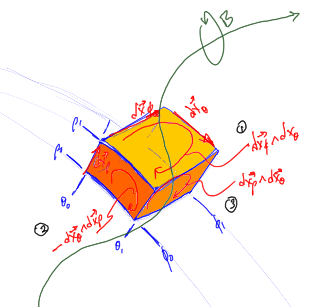
There is a geometric interpretation to these oriented area integrals, especially when written out explicitly in terms of the differentials along the parameterization directions. Pulling out a sign explicitly to match the geometry (as we had to also do for the line integrals in the two parameter volume element case), we can write this as

\begin{aligned}\int_{\partial V} d^2 \mathbf{x} \cdot B = -\int {\left.{{ \left( { d\mathbf{x}_\phi \wedge d\mathbf{x}_\theta } \right) \cdot B }}\right\vert}_{{\rho = \rho_0}}^{{\rho_1}} -\int{\left.{{ \left( { d\mathbf{x}_\rho \wedge d\mathbf{x}_\phi } \right) \cdot B }}\right\vert}_{{\theta = \theta_0}}^{{\theta_1}} -\int{\left.{{ \left( { d\mathbf{x}_\theta \wedge d\mathbf{x}_\rho } \right) \cdot B }}\right\vert}_{{\phi = \phi_0}}^{{\phi_1}}.\end{aligned} \hspace{\stretch{1}}(1.0.94)

When written out in this differential form, each of the respective area elements is an oriented area along one of the faces of the parameterization volume, much like the line integral that results from a two parameter volume curl integral. This is visualized in fig. 1.8. In this figure, faces (1) and (3) are “top faces”, those with signs matching the tops of the evaluation ranges eq. 1.0.94, whereas face (2) is a bottom face with a sign that is correspondingly reversed.

Fig 1.8. Boundary faces of a spherical parameterization region

Example: Minkowski hyperbolic-spherical polar parameterization of 3D subspace

Working with a three parameter volume element in a Minkowski space does not change much. For example in a 4D space with \left( {\mathbf{e}_4} \right)^2 = -1, we can employ a hyperbolic-spherical parameterization similar to that used above for the 4D Euclidean space

\begin{aligned}\mathbf{x}(x, \rho, \alpha, \phi)=\left\{ {x, \rho \sinh \alpha \cos\phi, \rho \sinh \alpha \sin\phi, \rho \cosh \alpha} \right\}=\mathbf{e}_1 x + \mathbf{e}_4 \rho \exp\left( { \mathbf{e}_4 \mathbf{e}_2 e^{\mathbf{e}_2 \mathbf{e}_3 \phi} \alpha } \right).\end{aligned} \hspace{\stretch{1}}(1.0.95)

This has tangent space basis elements

\begin{aligned}\begin{aligned}\mathbf{x}_\rho &= \sinh\alpha \left( { \cos\phi \mathbf{e}_2 + \sin\phi \mathbf{e}_3 } \right) + \cosh\alpha \mathbf{e}_4 = \mathbf{e}_4 \exp\left( {\mathbf{e}_4 \mathbf{e}_2 e^{\mathbf{e}_2 \mathbf{e}_3 \phi} \alpha} \right) \\ \mathbf{x}_\alpha &=\rho \cosh\alpha \left( { \cos\phi \mathbf{e}_2 + \sin\phi \mathbf{e}_3} \right) + \rho \sinh\alpha \mathbf{e}_4=\rho \mathbf{e}_2 e^{\mathbf{e}_2 \mathbf{e}_3 \phi} \exp\left( {-\mathbf{e}_4 \mathbf{e}_2 e^{\mathbf{e}_2 \mathbf{e}_3 \phi} \alpha} \right) \\ \mathbf{x}_\phi &=\rho \sinh\alpha \left( { \mathbf{e}_3 \cos\phi - \mathbf{e}_2 \sin\phi} \right) = \rho\sinh\alpha \mathbf{e}_3 e^{\mathbf{e}_2 \mathbf{e}_3 \phi}.\end{aligned}\end{aligned} \hspace{\stretch{1}}(1.0.96)

This is a normal basis, but again not orthonormal. Specifically, for i,j \in \left\{ {\rho, \theta, \phi} \right\} we have

\begin{aligned}\mathbf{x}_i \cdot \mathbf{x}_j =\begin{bmatrix}-1 & 0 & 0 \\ 0 & \rho^2 & 0 \\ 0 & 0 & \rho^2 \sinh^2 \alpha \end{bmatrix},\end{aligned} \hspace{\stretch{1}}(1.0.97)

where we see that the radial vector \mathbf{x}_\rho is timelike. We can form the dual basis again by inspection

\begin{aligned}\begin{aligned}\mathbf{x}_\rho &= -\mathbf{e}_4 \exp\left( {\mathbf{e}_4 \mathbf{e}_2 e^{\mathbf{e}_2 \mathbf{e}_3 \phi} \alpha} \right) \\ \mathbf{x}_\alpha &= \frac{1}{{\rho}} \mathbf{e}_2 e^{\mathbf{e}_2 \mathbf{e}_3 \phi} \exp\left( {-\mathbf{e}_4 \mathbf{e}_2 e^{\mathbf{e}_2 \mathbf{e}_3 \phi} \alpha} \right) \\ \mathbf{x}_\phi &= \frac{1}{{\rho\sinh\alpha}} \mathbf{e}_3 e^{\mathbf{e}_2 \mathbf{e}_3 \phi}.\end{aligned}\end{aligned} \hspace{\stretch{1}}(1.0.98)

The area elements are

\begin{aligned}\begin{aligned}\mathbf{x}_\alpha \wedge \mathbf{x}_\phi &=\rho^2 \sinh\alpha \left(-\mathbf{e}_4 \mathbf{e}_3 \sinh\alpha \cos\phi+\cosh\alpha \mathbf{e}_2 \mathbf{e}_3+\sinh\alpha \sin\phi \mathbf{e}_2 \mathbf{e}_4\right) \\ \mathbf{x}_\phi \wedge \mathbf{x}_\rho &=\rho \sinh\alpha \left(-\mathbf{e}_2 \mathbf{e}_3 \sinh\alpha-\mathbf{e}_2 \mathbf{e}_4 \cosh\alpha \sin\phi+\cosh\alpha \cos\phi \mathbf{e}_3 \mathbf{e}_4\right) \\ \mathbf{x}_\rho \wedge \mathbf{x}_\alpha &=-\mathbf{e}_4 \rho \left(\cos\phi \mathbf{e}_2+\sin\phi \mathbf{e}_3\right),\end{aligned}\end{aligned} \hspace{\stretch{1}}(1.0.99)

or

\begin{aligned}\begin{aligned}\mathbf{x}_\alpha \wedge \mathbf{x}_\phi &=\rho^2 \sinh\alpha \mathbf{e}_2 \mathbf{e}_3 \exp\left( { \mathbf{e}_4 \mathbf{e}_2 e^{-\mathbf{e}_2 \mathbf{e}_3 \phi} \alpha } \right) \\ \mathbf{x}_\phi \wedge \mathbf{x}_\rho &=\rho\sinh\alpha \mathbf{e}_3 \mathbf{e}_4 e^{\mathbf{e}_2 \mathbf{e}_3 \phi} \exp\left( {\mathbf{e}_4 \mathbf{e}_2 e^{\mathbf{e}_2 \mathbf{e}_3 \phi} \alpha} \right) \\ \mathbf{x}_\rho \wedge \mathbf{x}_\alpha &=-\mathbf{e}_4 \mathbf{e}_2 \rho e^{\mathbf{e}_2 \mathbf{e}_3 \phi}.\end{aligned}\end{aligned} \hspace{\stretch{1}}(1.0.100)

The volume element also reduces nicely, and is

\begin{aligned}\mathbf{x}_\rho \wedge \mathbf{x}_\alpha \wedge \mathbf{x}_\phi = \mathbf{e}_2 \mathbf{e}_3 \mathbf{e}_4 \rho^2 \sinh\alpha.\end{aligned} \hspace{\stretch{1}}(1.0.101)

The area and volume element reductions were once again messy, done in software using \nbref{sphericalSurfaceAndVolumeElementsMinkowski.nb}. However, we really only need eq. 1.0.96 to perform the Stokes integration.

Stokes theorem, four variable volume element parameterization

Volume elements for up to four parameters are likely of physical interest, with the four volume elements of interest for relativistic physics in \bigwedge^{3,1} spaces. For example, we may wish to use a parameterization u^1 = x, u^2 = y, u^3 = z, u^4 = \tau = c t, with a four volume

\begin{aligned}d^4 \mathbf{x}=d\mathbf{x}_x \wedge d\mathbf{x}_y \wedge d\mathbf{x}_z \wedge d\mathbf{x}_\tau,\end{aligned} \hspace{\stretch{1}}(1.102)

We follow the same procedure to calculate the corresponding boundary surface “area” element (with dimensions of volume in this case). This is

\begin{aligned}d^4 \mathbf{x} \cdot \left( { \boldsymbol{\partial} \wedge \mathbf{f} } \right) &= \left( { d^4 \mathbf{x} \cdot \mathbf{x}^i } \right) \cdot \partial_i \mathbf{f} \\ &= du^1 du^2 du^3 du^4\left( {\left( { \mathbf{x}_1 \wedge \mathbf{x}_2 \wedge \mathbf{x}_3 \wedge \mathbf{x}_4 } \right) \cdot \mathbf{x}^i } \right) \cdot \partial_i \mathbf{f} \\ &= du^1 du^2 du^3 du_4\left( {\left( { \mathbf{x}_1 \wedge \mathbf{x}_2 \wedge \mathbf{x}_3 } \right) {\delta_4}^i-\left( { \mathbf{x}_1 \wedge \mathbf{x}_2 \wedge \mathbf{x}_4 } \right) {\delta_3}^i+\left( { \mathbf{x}_1 \wedge \mathbf{x}_3 \wedge \mathbf{x}_4 } \right) {\delta_2}^i-\left( { \mathbf{x}_2 \wedge \mathbf{x}_3 \wedge \mathbf{x}_4 } \right) {\delta_1}^i} \right) \cdot \partial_i \mathbf{f} \\ &= du^1 du^2 du^3 du^4\left( { \left( { \mathbf{x}_1 \wedge \mathbf{x}_2 \wedge \mathbf{x}_3 } \right) \cdot \partial_4 \mathbf{f}-\left( { \mathbf{x}_1 \wedge \mathbf{x}_2 \wedge \mathbf{x}_4 } \right) \cdot \partial_3 \mathbf{f}+\left( { \mathbf{x}_1 \wedge \mathbf{x}_3 \wedge \mathbf{x}_4 } \right) \cdot \partial_2 \mathbf{f}-\left( { \mathbf{x}_2 \wedge \mathbf{x}_3 \wedge \mathbf{x}_4 } \right) \cdot \partial_1 \mathbf{f}} \right).\end{aligned} \hspace{\stretch{1}}(1.103)

Our boundary value surface element is therefore

\begin{aligned}d^3 \mathbf{x} = \mathbf{x}_1 \wedge \mathbf{x}_2 \wedge \mathbf{x}_3- \mathbf{x}_1 \wedge \mathbf{x}_2 \wedge \mathbf{x}_4+ \mathbf{x}_1 \wedge \mathbf{x}_3 \wedge \mathbf{x}_4- \mathbf{x}_2 \wedge \mathbf{x}_3 \wedge \mathbf{x}_4.\end{aligned} \hspace{\stretch{1}}(1.104)

where it is implied that this (and the dot products with \mathbf{f}) are evaluated on the boundaries of the integration ranges of the omitted index. This same boundary form can be used for vector, bivector and trivector variations of Stokes theorem.

Duality and its relation to the pseudoscalar.

Looking to eq. 1.0.181 of lemma 6, and scaling the wedge product \mathbf{a} \wedge \mathbf{b} by its absolute magnitude, we can express duality using that scaled bivector as a pseudoscalar for the plane that spans \left\{ {\mathbf{a}, \mathbf{b}} \right\}. Let’s introduce a subscript notation for such scaled blades

\begin{aligned}I_{\mathbf{a}\mathbf{b}} = \frac{\mathbf{a} \wedge \mathbf{b}}{\left\lvert {\mathbf{a} \wedge \mathbf{b}} \right\rvert}.\end{aligned} \hspace{\stretch{1}}(1.105)

This allows us to express the unit vector in the direction of \mathbf{a}^{*} as

\begin{aligned}\widehat{\mathbf{a}^{*}} = \hat{\mathbf{b}} \frac{\left\lvert {\mathbf{a} \wedge \mathbf{b}} \right\rvert}{\mathbf{a} \wedge \mathbf{b}}= \hat{\mathbf{b}} \frac{1}{{I_{\mathbf{a} \mathbf{b}}}}.\end{aligned} \hspace{\stretch{1}}(1.0.106)

Following the pattern of eq. 1.0.181, it is clear how to express the dual vectors for higher dimensional subspaces. For example

or for the unit vector in the direction of \mathbf{a}^{*},

\begin{aligned}\widehat{\mathbf{a}^{*}} = I_{\mathbf{b} \mathbf{c}} \frac{1}{{I_{\mathbf{a} \mathbf{b} \mathbf{c}} }}.\end{aligned}

Divergence theorem.

When the curl integral is a scalar result we are able to apply duality relationships to obtain the divergence theorem for the corresponding space. We will be able to show that a relationship of the following form holds

\begin{aligned}\int_V dV \boldsymbol{\nabla} \cdot \mathbf{f} = \int_{\partial V} dA_i \hat{\mathbf{n}}^i \cdot \mathbf{f}.\end{aligned} \hspace{\stretch{1}}(1.0.107)

Here \mathbf{f} is a vector, \hat{\mathbf{n}}^i is normal to the boundary surface, and dA_i is the area of this bounding surface element. We wish to quantify these more precisely, especially because the orientation of the normal vectors are metric dependent. Working a few specific examples will show the pattern nicely, but it is helpful to first consider some aspects of the general case.

First note that, for a scalar Stokes integral we are integrating the vector derivative curl of a blade F \in \bigwedge^{k-1} over a k-parameter volume element. Because the dimension of the space matches the number of parameters, the projection of the gradient onto the tangent space is exactly that gradient

\begin{aligned}\int_V d^k \mathbf{x} \cdot (\boldsymbol{\partial} \wedge F) =\int_V d^k \mathbf{x} \cdot (\boldsymbol{\nabla} \wedge F).\end{aligned} \hspace{\stretch{1}}(1.0.108)

Multiplication of F by the pseudoscalar will always produce a vector. With the introduction of such a dual vector, as in

\begin{aligned}F = I \mathbf{f},\end{aligned} \hspace{\stretch{1}}(1.0.108)

Stokes theorem takes the form

\begin{aligned}\int_V d^k \mathbf{x} \cdot {\left\langle{{\boldsymbol{\nabla} I \mathbf{f}}}\right\rangle}_{k}= \int_{\partial V} \left\langle{{ d^{k-1} \mathbf{x} I \mathbf{f}}}\right\rangle,\end{aligned} \hspace{\stretch{1}}(1.0.108)

or

\begin{aligned}\int_V \left\langle{{ d^k \mathbf{x} \boldsymbol{\nabla} I \mathbf{f}}}\right\rangle= \int_{\partial V} \left( { d^{k-1} \mathbf{x} I} \right) \cdot \mathbf{f},\end{aligned} \hspace{\stretch{1}}(1.0.108)

where we will see that the vector d^{k-1} \mathbf{x} I can roughly be characterized as a normal to the boundary surface. Using primes to indicate the scope of the action of the gradient, cyclic permutation within the scalar selection operator can be used to factor out the pseudoscalar

\begin{aligned}\int_V \left\langle{{ d^k \mathbf{x} \boldsymbol{\nabla} I \mathbf{f}}}\right\rangle &= \int_V \left\langle{{ \mathbf{f}' d^k \mathbf{x} \boldsymbol{\nabla}' I}}\right\rangle \\ &= \int_V {\left\langle{{ \mathbf{f}' d^k \mathbf{x} \boldsymbol{\nabla}'}}\right\rangle}_{k} I \\ &= \int_V(-1)^{k+1} d^k \mathbf{x} \left( { \boldsymbol{\nabla} \cdot \mathbf{f}} \right) I \\ &= (-1)^{k+1} I^2\int_V dV\left( { \boldsymbol{\nabla} \cdot \mathbf{f}} \right).\end{aligned} \hspace{\stretch{1}}(1.0.108)

The second last step uses lemma 8, and the last writes d^k \mathbf{x} = I^2 \left\lvert {d^k \mathbf{x}} \right\rvert = I^2 dV, where we have assumed (without loss of generality) that d^k \mathbf{x} has the same orientation as the pseudoscalar for the space. We also assume that the parameterization is non-degenerate over the integration volume (i.e. no d\mathbf{x}_i = 0), so the sign of this product cannot change.

Let’s now return to the normal vector d^{k-1} \mathbf{x} I. With d^{k-1} u_i = du^1 du^2 \cdots du^{i-1} du^{i+1} \cdots du^k (the i indexed differential omitted), and I_{ab\cdots c} = (\mathbf{x}_a \wedge \mathbf{x}_b \wedge \cdots \wedge \mathbf{x}_c)/\left\lvert {\mathbf{x}_a \wedge \mathbf{x}_b \wedge \cdots \wedge \mathbf{x}_c} \right\rvert, we have

\begin{aligned}\begin{aligned}d^{k-1} \mathbf{x} I&=d^{k-1} u_i \left( { \mathbf{x}_1 \wedge \mathbf{x}_2 \wedge \cdots \wedge \mathbf{x}_k} \right) \cdot \mathbf{x}^i I \\ &= I_{1 2 \cdots (k-1)} I \left\lvert {d\mathbf{x}_1 \wedge d\mathbf{x}_2 \wedge \cdots \wedge d\mathbf{x}_{k-1} } \right\rvert \\ &\quad -I_{1 \cdots (k-2) k} I \left\lvert {d\mathbf{x}_1 \wedge \cdots \wedge d\mathbf{x}_{k-2} \wedge d\mathbf{x}_k} \right\rvert+ \cdots\end{aligned}\end{aligned} \hspace{\stretch{1}}(1.0.113)

We’ve seen in eq. 1.0.106 and lemma 7 that the dual of vector \mathbf{a} with respect to the unit pseudoscalar I_{\mathbf{b} \cdots \mathbf{c} \mathbf{d}} in a subspace spanned by \left\{ {\mathbf{a}, \cdots \mathbf{c}, \mathbf{d}} \right\} is

\begin{aligned}\widehat{\mathbf{a}^{*}} = I_{\mathbf{b} \cdots \mathbf{c} \mathbf{d}} \frac{1}{{ I_{\mathbf{a} \cdots \mathbf{c} \mathbf{d}} }},\end{aligned} \hspace{\stretch{1}}(1.0.114)

or

\begin{aligned}\widehat{\mathbf{a}^{*}} I_{\mathbf{a} \cdots \mathbf{c} \mathbf{d}}^2=I_{\mathbf{b} \cdots \mathbf{c} \mathbf{d}}.\end{aligned} \hspace{\stretch{1}}(1.0.115)

This allows us to write

\begin{aligned}d^{k-1} \mathbf{x} I= I^2 \sum_i \widehat{\mathbf{x}^i} d{A'}_i\end{aligned} \hspace{\stretch{1}}(1.0.116)

where d{A'}_i = \pm dA_i, and dA_i is the area of the boundary area element normal to \mathbf{x}^i. Note that the I^2 term will now cancel cleanly from both sides of the divergence equation, taking both the metric and the orientation specific dependencies with it.

This leaves us with

\begin{aligned}\int_V dV \boldsymbol{\nabla} \cdot \mathbf{f} = (-1)^{k+1} \int_{\partial V} d{A'}_i \widehat{\mathbf{x}^i} \cdot \mathbf{f}.\end{aligned} \hspace{\stretch{1}}(1.0.117)

To spell out the details, we have to be very careful with the signs. However, that is a job best left for specific examples.

Example: 2D divergence theorem

Let’s start back at

\begin{aligned}\int_A \left\langle{{ d^2 \mathbf{x} \boldsymbol{\nabla} I \mathbf{f} }}\right\rangle = \int_{\partial A} \left( { d^1 \mathbf{x} I} \right) \cdot \mathbf{f}.\end{aligned} \hspace{\stretch{1}}(1.118)

On the left our integral can be rewritten as

\begin{aligned}\int_A \left\langle{{ d^2 \mathbf{x} \boldsymbol{\nabla} I \mathbf{f} }}\right\rangle &= -\int_A \left\langle{{ d^2 \mathbf{x} I \boldsymbol{\nabla} \mathbf{f} }}\right\rangle \\ &= -\int_A d^2 \mathbf{x} I \left( { \boldsymbol{\nabla} \cdot \mathbf{f} } \right) \\ &= - I^2 \int_A dA \boldsymbol{\nabla} \cdot \mathbf{f},\end{aligned} \hspace{\stretch{1}}(1.119)

where d^2 \mathbf{x} = I dA and we pick the pseudoscalar with the same orientation as the volume (area in this case) element I = (\mathbf{x}_1 \wedge \mathbf{x}_2)/\left\lvert {\mathbf{x}_1 \wedge \mathbf{x}_2} \right\rvert.

For the boundary form we have

\begin{aligned}d^1 \mathbf{x} = du^2 \left( { \mathbf{x}_1 \wedge \mathbf{x}_2 } \right) \cdot \mathbf{x}^1+ du^1 \left( { \mathbf{x}_1 \wedge \mathbf{x}_2 } \right) \cdot \mathbf{x}^2= -du^2 \mathbf{x}_2 +du^1 \mathbf{x}_1.\end{aligned} \hspace{\stretch{1}}(1.120)

The duality relations for the tangent space are

\begin{aligned}\begin{aligned}\mathbf{x}^2 &= \mathbf{x}_1 \frac{1}{{\mathbf{x}_2 \wedge \mathbf{x}_1}} \\ \mathbf{x}^1 &= \mathbf{x}_2 \frac{1}{{\mathbf{x}_1 \wedge \mathbf{x}_2}}\end{aligned},\end{aligned} \hspace{\stretch{1}}(1.0.121)

or

\begin{aligned}\begin{aligned}\widehat{\mathbf{x}^2} &= -\widehat{\mathbf{x}_1} \frac{1}{I} \\ \widehat{\mathbf{x}^1} &= \widehat{\mathbf{x}_2} \frac{1}{I}\end{aligned}.\end{aligned} \hspace{\stretch{1}}(1.0.122)

Back substitution into the line element gives

\begin{aligned}d^1 \mathbf{x} = -du^2 \left\lvert {\mathbf{x}_2} \right\rvert \widehat{\mathbf{x}_2}+du^1 \left\lvert {\mathbf{x}_1} \right\rvert \widehat{\mathbf{x}_1}=-du^2 \left\lvert {\mathbf{x}_2} \right\rvert \widehat{\mathbf{x}^1} I-du^1 \left\lvert {\mathbf{x}_1} \right\rvert \widehat{\mathbf{x}^2} I.\end{aligned} \hspace{\stretch{1}}(1.0.122)

Writing (no sum) du^i \left\lvert {\mathbf{x}_i} \right\rvert = ds_i, we have

\begin{aligned}d^1 \mathbf{x} I = -\left( { ds_2 \widehat{\mathbf{x}^1} +ds_1 \widehat{\mathbf{x}^2} } \right) I^2.\end{aligned} \hspace{\stretch{1}}(1.0.122)

This provides us a divergence and normal relationship, with -I^2 terms on each side that can be canceled. Restoring explicit range evaluation, that is

\begin{aligned}\int_A dA \boldsymbol{\nabla} \cdot \mathbf{f}=\int_{\Delta u^2} {\left.{{ ds_2 \widehat{\mathbf{x}^1} \cdot \mathbf{f}}}\right\vert}_{{\Delta u^1}}+ \int_{\Delta u^1} {\left.{{ ds_1 \widehat{\mathbf{x}^2} \cdot \mathbf{f}}}\right\vert}_{{\Delta u^2}}=\int_{\Delta u^2} {\left.{{ ds_2 \widehat{\mathbf{x}^1} \cdot \mathbf{f}}}\right\vert}_{{u^1(1)}}-\int_{\Delta u^2} {\left.{{ ds_2 \widehat{\mathbf{x}^1} \cdot \mathbf{f}}}\right\vert}_{{u^1(0)}}+ \int_{\Delta u^1} {\left.{{ ds_1 \widehat{\mathbf{x}^2} \cdot \mathbf{f}}}\right\vert}_{{u^2(0)}}- \int_{\Delta u^1} {\left.{{ ds_1 \widehat{\mathbf{x}^2} \cdot \mathbf{f}}}\right\vert}_{{u^2(0)}}.\end{aligned} \hspace{\stretch{1}}(1.0.122)

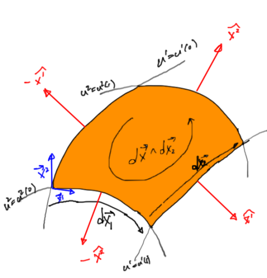
Let’s consider this graphically for an Euclidean metric as illustrated in fig. 1.9.

Fig 1.9. Normals on area element

We see that

  1. along u^2(0) the outwards normal is -\widehat{\mathbf{x}^2},
  2. along u^2(1) the outwards normal is \widehat{\mathbf{x}^2},
  3. along u^1(0) the outwards normal is -\widehat{\mathbf{x}^1}, and
  4. along u^1(1) the outwards normal is \widehat{\mathbf{x}^2}.

Writing that outwards normal as \hat{\mathbf{n}}, we have

\begin{aligned}\int_A dA \boldsymbol{\nabla} \cdot \mathbf{f}= \mathop{\rlap{\ensuremath{\mkern3.5mu\circlearrowright}}\int} ds \hat{\mathbf{n}} \cdot \mathbf{f}.\end{aligned} \hspace{\stretch{1}}(1.0.126)

Note that we can use the same algebraic notion of outward normal for non-Euclidean spaces, although cannot expect the geometry to look anything like that of the figure.

Example: 3D divergence theorem

As with the 2D example, let’s start back with

\begin{aligned}\int_V \left\langle{{ d^3 \mathbf{x} \boldsymbol{\nabla} I \mathbf{f} }}\right\rangle = \int_{\partial V} \left( { d^2 \mathbf{x} I} \right) \cdot \mathbf{f}.\end{aligned} \hspace{\stretch{1}}(1.127)

In a 3D space, the pseudoscalar commutes with all grades, so we have

\begin{aligned}\int_V \left\langle{{ d^3 \mathbf{x} \boldsymbol{\nabla} I \mathbf{f} }}\right\rangle=\int_V \left( { d^3 \mathbf{x} I } \right) \boldsymbol{\nabla} \cdot \mathbf{f}=I^2 \int_V dV \boldsymbol{\nabla} \cdot \mathbf{f},\end{aligned} \hspace{\stretch{1}}(1.128)

where d^3 \mathbf{x} I = dV I^2, and we have used a pseudoscalar with the same orientation as the volume element

\begin{aligned}\begin{aligned}I &= \widehat{ \mathbf{x}_{123} } \\ \mathbf{x}_{123} &= \mathbf{x}_1 \wedge \mathbf{x}_2 \wedge \mathbf{x}_3.\end{aligned}\end{aligned} \hspace{\stretch{1}}(1.0.129)

In the boundary integral our dual two form is

\begin{aligned}d^2 \mathbf{x} I= du^1 du^2 \mathbf{x}_1 \wedge \mathbf{x}_2+du^3 du^1 \mathbf{x}_3 \wedge \mathbf{x}_1+du^2 du^3 \mathbf{x}_2 \wedge \mathbf{x}_3= \left( { dA_{3} \widehat{ \mathbf{x}_{12} } \frac{1}{I}+dA_{2} \widehat{ \mathbf{x}_{31} } \frac{1}{I}+dA_{1} \widehat{ \mathbf{x}_{23} } \frac{1}{I}} \right) I^2,\end{aligned} \hspace{\stretch{1}}(1.0.129)

where \mathbf{x}_{ij} = \mathbf{x}_i \wedge \mathbf{x}_j, and

\begin{aligned}\begin{aligned}dA_1 &= \left\lvert {d\mathbf{x}_2 \wedge d\mathbf{x}_3} \right\rvert \\ dA_2 &= \left\lvert {d\mathbf{x}_3 \wedge d\mathbf{x}_1} \right\rvert \\ dA_3 &= \left\lvert {d\mathbf{x}_1 \wedge d\mathbf{x}_2} \right\rvert.\end{aligned}\end{aligned} \hspace{\stretch{1}}(1.0.131)

Observe that we can do a cyclic permutation of a 3 blade without any change of sign, for example

\begin{aligned}\mathbf{x}_1 \wedge \mathbf{x}_2 \wedge \mathbf{x}_3 =-\mathbf{x}_2 \wedge \mathbf{x}_1 \wedge \mathbf{x}_3 =\mathbf{x}_2 \wedge \mathbf{x}_3 \wedge \mathbf{x}_1.\end{aligned} \hspace{\stretch{1}}(1.0.132)

Because of this we can write the dual two form as we expressed the normals in lemma 7

\begin{aligned}d^2 \mathbf{x} I = \left( { dA_1 \widehat{\mathbf{x}_{23}} \frac{1}{{\widehat{\mathbf{x}_{123}}}} + dA_2 \widehat{\mathbf{x}_{31}} \frac{1}{{\widehat{\mathbf{x}_{231}}}} + dA_3 \widehat{\mathbf{x}_{12}} \frac{1}{{\widehat{\mathbf{x}_{312}}}}} \right) I^2=\left( { dA_1 \widehat{\mathbf{x}^1}+dA_2 \widehat{\mathbf{x}^2}+dA_3 \widehat{\mathbf{x}^3} } \right) I^2.\end{aligned} \hspace{\stretch{1}}(1.0.132)

We can now state the 3D divergence theorem, canceling out the metric and orientation dependent term I^2 on both sides

\begin{aligned}\int_V dV \boldsymbol{\nabla} \cdot \mathbf{f}=\int dA \hat{\mathbf{n}} \cdot \mathbf{f},\end{aligned} \hspace{\stretch{1}}(1.0.134)

where (sums implied)

\begin{aligned}dA \hat{\mathbf{n}} = dA_i \widehat{\mathbf{x}^i},\end{aligned} \hspace{\stretch{1}}(1.0.135)

and

\begin{aligned}\begin{aligned}{\left.{{\hat{\mathbf{n}}}}\right\vert}_{{u^i = u^i(1)}} &= \widehat{\mathbf{x}^i} \\ {\left.{{\hat{\mathbf{n}}}}\right\vert}_{{u^i = u^i(0)}} &= -\widehat{\mathbf{x}^i}\end{aligned}.\end{aligned} \hspace{\stretch{1}}(1.0.136)

The outwards normals at the upper integration ranges of a three parameter surface are depicted in fig. 1.10.

Fig 1.10. Outwards normals on volume at upper integration ranges.

This sign alternation originates with the two form elements \left( {d\mathbf{x}_i \wedge d\mathbf{x}_j} \right) \cdot F from the Stokes boundary integral, which were explicitly evaluated at the endpoints of the integral. That is, for k \ne i,j,

\begin{aligned}\int_{\partial V} \left( { d\mathbf{x}_i \wedge d\mathbf{x}_j } \right) \cdot F\equiv\int_{\Delta u^i} \int_{\Delta u^j} {\left.{{\left( { \left( { d\mathbf{x}_i \wedge d\mathbf{x}_j } \right) \cdot F } \right)}}\right\vert}_{{u^k = u^k(1)}}-{\left.{{\left( { \left( { d\mathbf{x}_i \wedge d\mathbf{x}_j } \right) \cdot F } \right)}}\right\vert}_{{u^k = u^k(0)}}\end{aligned} \hspace{\stretch{1}}(1.0.137)

In the context of the divergence theorem, this means that we are implicitly requiring the dot products \widehat{\mathbf{x}^k} \cdot \mathbf{f} to be evaluated specifically at the end points of the integration where u^k = u^k(1), u^k = u^k(0), accounting for the alternation of sign required to describe the normals as uniformly outwards.

Example: 4D divergence theorem

Applying Stokes theorem to a trivector T = I \mathbf{f} in the 4D case we find

\begin{aligned}-I^2 \int_V d^4 x \boldsymbol{\nabla} \cdot \mathbf{f} = \int_{\partial V} \left( { d^3 \mathbf{x} I} \right) \cdot \mathbf{f}.\end{aligned} \hspace{\stretch{1}}(1.138)

Here the pseudoscalar has been picked to have the same orientation as the hypervolume element d^4 \mathbf{x} = I d^4 x. Writing \mathbf{x}_{ij \cdots k} = \mathbf{x}_i \wedge \mathbf{x}_j \wedge \cdots \mathbf{x}_k the dual of the three form is

\begin{aligned}d^3 \mathbf{x} I &= \left( { du^1 du^2 du^3 \mathbf{x}_{123}-du^1 du^2 du^4 \mathbf{x}_{124}+du^1 du^3 du^4 \mathbf{x}_{134}-du^2 du^3 du^4 \mathbf{x}_{234}} \right) I \\ &= \left( { dA^{123} \widehat{ \mathbf{x}_{123} } -dA^{124} \widehat{ \mathbf{x}_{124} } +dA^{134} \widehat{ \mathbf{x}_{134} } -dA^{234} \widehat{ \mathbf{x}_{234} }} \right) I \\ &= \left( { dA^{123} \widehat{ \mathbf{x}_{123} } \frac{1}{{\widehat{\mathbf{x}_{1234} }}} -dA^{124} \widehat{ \mathbf{x}_{124} } \frac{1}{{\widehat{\mathbf{x}_{1234} }}} +dA^{134} \widehat{ \mathbf{x}_{134} } \frac{1}{{\widehat{\mathbf{x}_{1234} }}} -dA^{234} \widehat{ \mathbf{x}_{234} } \frac{1}{{\widehat{\mathbf{x}_{1234} }}}} \right) I^2 \\ &= -\left( { dA^{123} \widehat{ \mathbf{x}_{123} } \frac{1}{{\widehat{\mathbf{x}_{4123} }}} +dA^{124} \widehat{ \mathbf{x}_{124} } \frac{1}{{\widehat{\mathbf{x}_{3412} }}} +dA^{134} \widehat{ \mathbf{x}_{134} } \frac{1}{{\widehat{\mathbf{x}_{2341} }}} +dA^{234} \widehat{ \mathbf{x}_{234} } \frac{1}{{\widehat{\mathbf{x}_{1234} }}}} \right) I^2 \\ &= -\left( { dA^{123} \widehat{ \mathbf{x}_{123} } \frac{1}{{\widehat{\mathbf{x}_{4123} }}} +dA^{124} \widehat{ \mathbf{x}_{412} } \frac{1}{{\widehat{\mathbf{x}_{3412} }}} +dA^{134} \widehat{ \mathbf{x}_{341} } \frac{1}{{\widehat{\mathbf{x}_{2341} }}} +dA^{234} \widehat{ \mathbf{x}_{234} } \frac{1}{{\widehat{\mathbf{x}_{1234} }}}} \right) I^2 \\ &= -\left( { dA^{123} \widehat{ \mathbf{x}^{4} } +dA^{124} \widehat{ \mathbf{x}^{3} } +dA^{134} \widehat{ \mathbf{x}^{2} } +dA^{234} \widehat{ \mathbf{x}^{1} } } \right) I^2\end{aligned} \hspace{\stretch{1}}(1.139)

Here, we’ve written

\begin{aligned}dA^{ijk} = \left\lvert { d\mathbf{x}_i \wedge d\mathbf{x}_j \wedge d\mathbf{x}_k } \right\rvert.\end{aligned} \hspace{\stretch{1}}(1.140)

Observe that the dual representation nicely removes the alternation of sign that we had in the Stokes theorem boundary integral, since each alternation of the wedged vectors in the pseudoscalar changes the sign once.

As before, we define the outwards normals as \hat{\mathbf{n}} = \pm \widehat{\mathbf{x}^i} on the upper and lower integration ranges respectively. The scalar area elements on these faces can be written in a dual form

\begin{aligned}\begin{aligned} dA_4 &= dA^{123} \\ dA_3 &= dA^{124} \\ dA_2 &= dA^{134} \\ dA_1 &= dA^{234} \end{aligned},\end{aligned} \hspace{\stretch{1}}(1.0.141)

so that the 4D divergence theorem looks just like the 2D and 3D cases

\begin{aligned}\int_V d^4 x \boldsymbol{\nabla} \cdot \mathbf{f} = \int_{\partial V} d^3 x \hat{\mathbf{n}} \cdot \mathbf{f}.\end{aligned} \hspace{\stretch{1}}(1.0.142)

Here we define the volume scaled normal as

\begin{aligned}d^3 x \hat{\mathbf{n}} = dA_i \widehat{\mathbf{x}^i}.\end{aligned} \hspace{\stretch{1}}(1.0.143)

As before, we have made use of the implicit fact that the three form (and it’s dot product with \mathbf{f}) was evaluated on the boundaries of the integration region, with a toggling of sign on the lower limit of that evaluation that is now reflected in what we have defined as the outwards normal.

We also obtain explicit instructions from this formalism how to compute the “outwards” normal for this surface in a 4D space (unit scaling of the dual basis elements), something that we cannot compute using any sort of geometrical intuition. For free we’ve obtained a result that applies to both Euclidean and Minkowski (or other non-Euclidean) spaces.

Volume integral coordinate representations

It may be useful to formulate the curl integrals in tensor form. For vectors \mathbf{f}, and bivectors B, the coordinate representations of those differential forms (\cref{pr:stokesTheoremGeometricAlgebraII:1}) are

\begin{aligned}d^2 \mathbf{x} \cdot \left( { \boldsymbol{\partial} \wedge \mathbf{f} } \right)=- d^2 u \epsilon^{ a b } \partial_a f_b\end{aligned} \hspace{\stretch{1}}(1.0.144a)

\begin{aligned}d^3 \mathbf{x} \cdot \left( { \boldsymbol{\partial} \wedge \mathbf{f} } \right)=-d^3 u \epsilon^{a b c} \mathbf{x}_a \partial_b f_{c}\end{aligned} \hspace{\stretch{1}}(1.0.144b)

\begin{aligned}d^4 \mathbf{x} \cdot \left( { \boldsymbol{\partial} \wedge \mathbf{f} } \right)=-\frac{1}{2} d^4 u \epsilon^{a b c d} \mathbf{x}_a \wedge \mathbf{x}_b \partial_{c} f_{d}\end{aligned} \hspace{\stretch{1}}(1.0.144c)

\begin{aligned}d^3 \mathbf{x} \cdot \left( { \boldsymbol{\partial} \wedge B } \right)=-\frac{1}{2}d^3 u \epsilon^{a b c} \partial_a B_{b c}\end{aligned} \hspace{\stretch{1}}(1.0.144d)

\begin{aligned}d^4 \mathbf{x} \cdot \left( { \boldsymbol{\partial} \wedge B } \right)=-\frac{1}{2} d^4 u \epsilon^{a b c d} \mathbf{x}_a \partial_b B_{cd}\end{aligned} \hspace{\stretch{1}}(1.0.144e)

\begin{aligned}d^4 \mathbf{x} \cdot \left( { \boldsymbol{\partial} \wedge T } \right)=-d^4 u\left( {\partial_4 T_{123}-\partial_3 T_{124}+\partial_2 T_{134}-\partial_1 T_{234}} \right).\end{aligned} \hspace{\stretch{1}}(1.0.144f)

Here the bivector B and trivector T is expressed in terms of their curvilinear components on the tangent space

\begin{aligned}B = \frac{1}{2} \mathbf{x}^i \wedge \mathbf{x}^j B_{ij} + B_\perp\end{aligned} \hspace{\stretch{1}}(1.0.145a)

\begin{aligned}T = \frac{1}{{3!}} \mathbf{x}^i \wedge \mathbf{x}^j \wedge \mathbf{x}^k T_{ijk} + T_\perp,\end{aligned} \hspace{\stretch{1}}(1.0.145b)

where

\begin{aligned}B_{ij} = \mathbf{x}_j \cdot \left( { \mathbf{x}_i \cdot B } \right) = -B_{ji}.\end{aligned} \hspace{\stretch{1}}(1.0.146a)

\begin{aligned}T_{ijk} = \mathbf{x}_k \cdot \left( { \mathbf{x}_j \cdot \left( { \mathbf{x}_i \cdot B } \right)} \right).\end{aligned} \hspace{\stretch{1}}(1.0.146b)

For the trivector components are also antisymmetric, changing sign with any interchange of indices.

Note that eq. 1.0.144d and eq. 1.0.144f appear much different on the surface, but both have the same structure. This can be seen by writing for former as

\begin{aligned}d^3 \mathbf{x} \cdot \left( { \boldsymbol{\partial} \wedge B } \right)=-d^3 u\left( { \partial_1 B_{2 3} + \partial_2 B_{3 1} + \partial_3 B_{1 2}} \right)=-d^3 u\left( { \partial_3 B_{1 2} - \partial_2 B_{1 3} + \partial_1 B_{2 3}} \right).\end{aligned} \hspace{\stretch{1}}(1.0.146b)

In both of these we have an alternation of sign, where the tensor index skips one of the volume element indices is sequence. We’ve seen in the 4D divergence theorem that this alternation of sign can be related to a duality transformation.

In integral form (no sum over indexes i in du^i terms), these are

\begin{aligned}\int d^2 \mathbf{x} \cdot \left( { \boldsymbol{\partial} \wedge \mathbf{f} } \right)=- \epsilon^{ a b } \int {\left.{{du^b f_b}}\right\vert}_{{\Delta u^a}}\end{aligned} \hspace{\stretch{1}}(1.0.148a)

\begin{aligned}\int d^3 \mathbf{x} \cdot \left( { \boldsymbol{\partial} \wedge \mathbf{f} } \right)=-\epsilon^{a b c} \int du^a du^c{\left.{{\mathbf{x}_a f_{c}}}\right\vert}_{{\Delta u^b}}\end{aligned} \hspace{\stretch{1}}(1.0.148b)

\begin{aligned}\int d^4 \mathbf{x} \cdot \left( { \boldsymbol{\partial} \wedge \mathbf{f} } \right)=-\frac{1}{2} \epsilon^{a b c d} \int du^a du^b du^d{\left.{{\mathbf{x}_a \wedge \mathbf{x}_b f_{d}}}\right\vert}_{{\Delta u^c}}\end{aligned} \hspace{\stretch{1}}(1.0.148c)

\begin{aligned}\int d^3 \mathbf{x} \cdot \left( { \boldsymbol{\partial} \wedge B } \right)=-\frac{1}{2}\epsilon^{a b c} \int du^b du^c{\left.{{B_{b c}}}\right\vert}_{{\Delta u^a}}\end{aligned} \hspace{\stretch{1}}(1.0.148d)

\begin{aligned}\int d^4 \mathbf{x} \cdot \left( { \boldsymbol{\partial} \wedge B } \right)=-\frac{1}{2} \epsilon^{a b c d} \int du^a du^c du^d{\left.{{\mathbf{x}_a B_{cd}}}\right\vert}_{{\Delta u^b}}\end{aligned} \hspace{\stretch{1}}(1.0.148e)

\begin{aligned}\int d^4 \mathbf{x} \cdot \left( { \boldsymbol{\partial} \wedge T } \right)=-\int \left( {du^1 du^2 du^3 {\left.{{T_{123}}}\right\vert}_{{\Delta u^4}}-du^1 du^2 du^4 {\left.{{T_{124}}}\right\vert}_{{\Delta u^3}}+du^1 du^3 du^4 {\left.{{T_{134}}}\right\vert}_{{\Delta u^2}}-du^2 du^3 du^4 {\left.{{T_{234}}}\right\vert}_{{\Delta u^1}}} \right).\end{aligned} \hspace{\stretch{1}}(1.0.148f)

Of these, I suspect that only eq. 1.0.148a and eq. 1.0.148d are of use.

Final remarks

Because we have used curvilinear coordinates from the get go, we have arrived naturally at a formulation that works for both Euclidean and non-Euclidean geometries, and have demonstrated that Stokes (and the divergence theorem) holds regardless of the geometry or the parameterization. We also know explicitly how to formulate both theorems for any parameterization that we choose, something much more valuable than knowledge that this is possible.

For the divergence theorem we have introduced the concept of outwards normal (for example in 3D, eq. 1.0.136), which still holds for non-Euclidean geometries. We may not be able to form intuitive geometrical interpretations for these normals, but do have an algebraic description of them.

Appendix

Problems

Question: Expand volume elements in coordinates

Show that the coordinate representation for the volume element dotted with the curl can be represented as a sum of antisymmetric terms. That is

  • (a)Prove eq. 1.0.144a
  • (b)Prove eq. 1.0.144b
  • (c)Prove eq. 1.0.144c
  • (d)Prove eq. 1.0.144d
  • (e)Prove eq. 1.0.144e
  • (f)Prove eq. 1.0.144f

Answer

(a) Two parameter volume, curl of vector

\begin{aligned}d^2 \mathbf{x} \cdot \left( \boldsymbol{\partial} \wedge \mathbf{f} \right) &= d^2 u\Bigl( { \left( \mathbf{x}_1 \wedge \mathbf{x}_2 \right) \cdot \mathbf{x}^i } \Bigr) \cdot \partial_i \mathbf{f} \\ &= d^2 u \left( \mathbf{x}_1 \cdot \partial_2 \mathbf{f}-\mathbf{x}_2 \cdot \partial_1 \mathbf{f} \right) \\ &= d^2 u\left( \partial_2 f_1-\partial_1 f_2 \right) \\ &= - d^2 u \epsilon^{ab} \partial_{a} f_{b}. \qquad\square\end{aligned} \hspace{\stretch{1}}(1.149)

(b) Three parameter volume, curl of vector

\begin{aligned}d^3 \mathbf{x} \cdot \left( { \boldsymbol{\partial} \wedge \mathbf{f} } \right) &= d^3 u\Bigl( { \left( { \mathbf{x}_1 \wedge \mathbf{x}_2 \wedge \mathbf{x}_3 } \right) \cdot \mathbf{x}^i } \Bigr) \cdot \partial_i \mathbf{f} \\ &= d^3 u\Bigl( { \left( { \mathbf{x}_1 \wedge \mathbf{x}_2 } \right) \cdot \partial_3 \mathbf{f}+\left( { \mathbf{x}_3 \wedge \mathbf{x}_1 } \right) \cdot \partial_2 \mathbf{f}+\left( { \mathbf{x}_2 \wedge \mathbf{x}_3 } \right) \cdot \partial_1 \mathbf{f}} \Bigr) \\ &= d^3 u\Bigl( {\left( { \mathbf{x}_1 \partial_3 \mathbf{f} \cdot \mathbf{x}_2 -\mathbf{x}_2 \partial_3 \mathbf{f} \cdot \mathbf{x}_1 } \right)+\left( { \mathbf{x}_3 \partial_2 \mathbf{f} \cdot \mathbf{x}_1 -\mathbf{x}_1 \partial_2 \mathbf{f} \cdot \mathbf{x}_3 } \right)+\left( { \mathbf{x}_2 \partial_1 \mathbf{f} \cdot \mathbf{x}_3 -\mathbf{x}_3 \partial_1 \mathbf{f} \cdot \mathbf{x}_2 } \right)} \Bigr) \\ &= d^3 u\Bigl( {\mathbf{x}_1 \left( { -\partial_2 \mathbf{f} \cdot \mathbf{x}_3 + \partial_3 \mathbf{f} \cdot \mathbf{x}_2 } \right)+\mathbf{x}_2 \left( { -\partial_3 \mathbf{f} \cdot \mathbf{x}_1 + \partial_1 \mathbf{f} \cdot \mathbf{x}_3 } \right)+\mathbf{x}_3 \left( { -\partial_1 \mathbf{f} \cdot \mathbf{x}_2 + \partial_2 \mathbf{f} \cdot \mathbf{x}_1 } \right)} \Bigr) \\ &= d^3 u\Bigl( {\mathbf{x}_1 \left( { -\partial_2 f_3 + \partial_3 f_2 } \right)+\mathbf{x}_2 \left( { -\partial_3 f_1 + \partial_1 f_3 } \right)+\mathbf{x}_3 \left( { -\partial_1 f_2 + \partial_2 f_1 } \right)} \Bigr) \\ &= - d^3 u \epsilon^{abc} \partial_b f_c. \qquad\square\end{aligned} \hspace{\stretch{1}}(1.150)

(c) Four parameter volume, curl of vector

\begin{aligned}\begin{aligned}d^4 \mathbf{x} \cdot \left( { \boldsymbol{\partial} \wedge \mathbf{f} } \right)&=d^4 u\Bigl( { \left( { \mathbf{x}_1 \wedge \mathbf{x}_2 \wedge \mathbf{x}_3 \wedge \mathbf{x}_4 } \right) \cdot \mathbf{x}^i } \Bigr) \cdot \partial_i \mathbf{f} \\ &=d^4 u\Bigl( {\left( { \mathbf{x}_1 \wedge \mathbf{x}_2 \wedge \mathbf{x}_3 } \right) \cdot \partial_4 \mathbf{f}-\left( { \mathbf{x}_1 \wedge \mathbf{x}_2 \wedge \mathbf{x}_4 } \right) \cdot \partial_3 \mathbf{f}+\left( { \mathbf{x}_1 \wedge \mathbf{x}_3 \wedge \mathbf{x}_4 } \right) \cdot \partial_2 \mathbf{f}-\left( { \mathbf{x}_2 \wedge \mathbf{x}_3 \wedge \mathbf{x}_4 } \right) \cdot \partial_1 \mathbf{f}} \Bigr) \\ &=d^4 u\Bigl( { \\ &\quad\quad \left( { \mathbf{x}_1 \wedge \mathbf{x}_2 } \right) \mathbf{x}_3 \cdot \partial_4 \mathbf{f}-\left( { \mathbf{x}_1 \wedge \mathbf{x}_3 } \right) \mathbf{x}_2 \cdot \partial_4 \mathbf{f}+\left( { \mathbf{x}_2 \wedge \mathbf{x}_3 } \right) \mathbf{x}_1 \cdot \partial_4 \mathbf{f} \\ &\quad-\left( { \mathbf{x}_1 \wedge \mathbf{x}_2 } \right) \mathbf{x}_4 \cdot \partial_3 \mathbf{f}+\left( { \mathbf{x}_1 \wedge \mathbf{x}_4 } \right) \mathbf{x}_2 \cdot \partial_3 \mathbf{f}-\left( { \mathbf{x}_2 \wedge \mathbf{x}_4 } \right) \mathbf{x}_1 \cdot \partial_3 \mathbf{f} \\ &\quad+ \left( { \mathbf{x}_1 \wedge \mathbf{x}_3 } \right) \mathbf{x}_4 \cdot \partial_2 \mathbf{f}-\left( { \mathbf{x}_1 \wedge \mathbf{x}_4 } \right) \mathbf{x}_3 \cdot \partial_2 \mathbf{f}+\left( { \mathbf{x}_3 \wedge \mathbf{x}_4 } \right) \mathbf{x}_1 \cdot \partial_2 \mathbf{f} \\ &\quad-\left( { \mathbf{x}_2 \wedge \mathbf{x}_3 } \right) \mathbf{x}_4 \cdot \partial_1 \mathbf{f}+\left( { \mathbf{x}_2 \wedge \mathbf{x}_4 } \right) \mathbf{x}_3 \cdot \partial_1 \mathbf{f}-\left( { \mathbf{x}_3 \wedge \mathbf{x}_4 } \right) \mathbf{x}_2 \cdot \partial_1 \mathbf{f} \\ &\qquad} \Bigr) \\ &=d^4 u\Bigl( {\mathbf{x}_1 \wedge \mathbf{x}_2 \partial_{[4} f_{3]}+\mathbf{x}_1 \wedge \mathbf{x}_3 \partial_{[2} f_{4]}+\mathbf{x}_1 \wedge \mathbf{x}_4 \partial_{[3} f_{2]}+\mathbf{x}_2 \wedge \mathbf{x}_3 \partial_{[4} f_{1]}+\mathbf{x}_2 \wedge \mathbf{x}_4 \partial_{[1} f_{3]}+\mathbf{x}_3 \wedge \mathbf{x}_4 \partial_{[2} f_{1]}} \Bigr) \\ &=- \frac{1}{2} d^4 u \epsilon^{abcd} \mathbf{x}_a \wedge \mathbf{x}_b \partial_{c} f_{d}. \qquad\square\end{aligned}\end{aligned} \hspace{\stretch{1}}(1.0.151)

(d) Three parameter volume, curl of bivector

\begin{aligned}\begin{aligned}d^3 \mathbf{x} \cdot \left( { \boldsymbol{\partial} \wedge B } \right)&=d^3 u\Bigl( { \left( { \mathbf{x}_1 \wedge \mathbf{x}_2 \wedge \mathbf{x}_3 } \right) \cdot \mathbf{x}^i } \Bigr) \cdot \partial_i B \\ &=d^3 u\Bigl( { \left( { \mathbf{x}_1 \wedge \mathbf{x}_2 } \right) \cdot \partial_3 B+\left( { \mathbf{x}_3 \wedge \mathbf{x}_1 } \right) \cdot \partial_2 B+\left( { \mathbf{x}_2 \wedge \mathbf{x}_3 } \right) \cdot \partial_1 B} \Bigr) \\ &=\frac{1}{2} d^3 u\Bigl( { \mathbf{x}_1 \cdot \left( { \mathbf{x}_2 \cdot \partial_3 B } \right) -\mathbf{x}_2 \cdot \left( { \mathbf{x}_1 \cdot \partial_3 B } \right) \\ &\qquad +\mathbf{x}_3 \cdot \left( { \mathbf{x}_1 \cdot \partial_2 B } \right) -\mathbf{x}_1 \cdot \left( { \mathbf{x}_3 \cdot \partial_2 B } \right) \\ &\qquad +\mathbf{x}_2 \cdot \left( { \mathbf{x}_3 \cdot \partial_1 B } \right) -\mathbf{x}_3 \cdot \left( { \mathbf{x}_2 \cdot \partial_1 B } \right)} \Bigr) \\ &=\frac{1}{2} d^3 u\Bigl( { \mathbf{x}_1 \cdot \left( { \mathbf{x}_2 \cdot \partial_3 B - \mathbf{x}_3 \cdot \partial_2 B } \right) \\ &\qquad +\mathbf{x}_2 \cdot \left( { \mathbf{x}_3 \cdot \partial_1 B - \mathbf{x}_1 \cdot \partial_3 B } \right) \\ &\qquad +\mathbf{x}_3 \cdot \left( { \mathbf{x}_1 \cdot \partial_2 B - \mathbf{x}_2 \cdot \partial_1 B } \right)} \Bigr) \\ &=\frac{1}{2} d^3 u\Bigl( {\mathbf{x}_1 \cdot \left( { \partial_3 \left( { \mathbf{x}_2 \cdot B} \right) - \partial_2 \left( { \mathbf{x}_3 \cdot B} \right) } \right) \\ &\qquad +\mathbf{x}_2 \cdot \left( { \partial_1 \left( { \mathbf{x}_3 \cdot B} \right) - \partial_3 \left( { \mathbf{x}_1 \cdot B} \right) } \right) \\ &\qquad +\mathbf{x}_3 \cdot \left( { \partial_2 \left( { \mathbf{x}_1 \cdot B} \right) - \partial_1 \left( { \mathbf{x}_2 \cdot B} \right) } \right)} \Bigr) \\ &=\frac{1}{2} d^3 u\Bigl( {\partial_2 \left( { \mathbf{x}_3 \cdot \left( { \mathbf{x}_1 \cdot B} \right) } \right) - \partial_3 \left( { \mathbf{x}_2 \cdot \left( { \mathbf{x}_1 \cdot B} \right) } \right) \\ &\qquad+ \partial_3 \left( { \mathbf{x}_1 \cdot \left( { \mathbf{x}_2 \cdot B} \right) } \right) - \partial_1 \left( { \mathbf{x}_3 \cdot \left( { \mathbf{x}_2 \cdot B} \right) } \right) \\ &\qquad+ \partial_1 \left( { \mathbf{x}_2 \cdot \left( { \mathbf{x}_3 \cdot B} \right) } \right) - \partial_2 \left( { \mathbf{x}_1 \cdot \left( { \mathbf{x}_3 \cdot B} \right) } \right)} \Bigr) \\ &=\frac{1}{2} d^3 u\Bigl( {\partial_2 B_{13} - \partial_3 B_{12}+\partial_3 B_{21} - \partial_1 B_{23}+\partial_1 B_{32} - \partial_2 B_{31}} \Bigr) \\ &=d^3 u\Bigl( {\partial_2 B_{13}+\partial_3 B_{21}+\partial_1 B_{32}} \Bigr) \\ &= - \frac{1}{2} d^3 u \epsilon^{abc} \partial_a B_{bc}. \qquad\square\end{aligned}\end{aligned} \hspace{\stretch{1}}(1.0.152)

(e) Four parameter volume, curl of bivector

To start, we require lemma 3. For convenience lets also write our wedge products as a single indexed quantity, as in \mathbf{x}_{abc} for \mathbf{x}_a \wedge \mathbf{x}_b \wedge \mathbf{x}_c. The expansion is

\begin{aligned}\begin{aligned}d^4 \mathbf{x} \cdot \left( \boldsymbol{\partial} \wedge B \right) &= d^4 u \left( \mathbf{x}_{1234} \cdot \mathbf{x}^i \right) \cdot \partial_i B \\ &= d^4 u\left( \mathbf{x}_{123} \cdot \partial_4 B - \mathbf{x}_{124} \cdot \partial_3 B + \mathbf{x}_{134} \cdot \partial_2 B - \mathbf{x}_{234} \cdot \partial_1 B \right) \\ &= d^4 u \Bigl( \mathbf{x}_1 \left( \mathbf{x}_{23} \cdot \partial_4 B \right) + \mathbf{x}_2 \left( \mathbf{x}_{32} \cdot \partial_4 B \right) + \mathbf{x}_3 \left( \mathbf{x}_{12} \cdot \partial_4 B \right) \\ &\qquad - \mathbf{x}_1 \left( \mathbf{x}_{24} \cdot \partial_3 B \right) - \mathbf{x}_2 \left( \mathbf{x}_{41} \cdot \partial_3 B \right) - \mathbf{x}_4 \left( \mathbf{x}_{12} \cdot \partial_3 B \right) \\ &\qquad + \mathbf{x}_1 \left( \mathbf{x}_{34} \cdot \partial_2 B \right) + \mathbf{x}_3 \left( \mathbf{x}_{41} \cdot \partial_2 B \right) + \mathbf{x}_4 \left( \mathbf{x}_{13} \cdot \partial_2 B \right) \\ &\qquad - \mathbf{x}_2 \left( \mathbf{x}_{34} \cdot \partial_1 B \right) - \mathbf{x}_3 \left( \mathbf{x}_{42} \cdot \partial_1 B \right) - \mathbf{x}_4 \left( \mathbf{x}_{23} \cdot \partial_1 B \right)} \Bigr) \\ &= d^4 u \Bigl( \mathbf{x}_1 \left( \mathbf{x}_{23} \cdot \partial_4 B + \mathbf{x}_{42} \cdot \partial_3 B + \mathbf{x}_{34} \cdot \partial_2 B \right) \\ &\qquad + \mathbf{x}_2 \left( \mathbf{x}_{32} \cdot \partial_4 B + \mathbf{x}_{14} \cdot \partial_3 B + \mathbf{x}_{43} \cdot \partial_1 B \right) \\ &\qquad + \mathbf{x}_3 \left( \mathbf{x}_{12} \cdot \partial_4 B + \mathbf{x}_{41} \cdot \partial_2 B + \mathbf{x}_{24} \cdot \partial_1 B \right) \\ &\qquad + \mathbf{x}_4 \left( \mathbf{x}_{21} \cdot \partial_3 B + \mathbf{x}_{13} \cdot \partial_2 B + \mathbf{x}_{32} \cdot \partial_1 B \right)} \Bigr) \\ &= - \frac{1}{2} d^4 u \epsilon^{a b c d} \mathbf{x}_a \partial_b B_{c d}. \qquad\square\end{aligned}\end{aligned} \hspace{\stretch{1}}(1.0.153)

This last step uses an intermediate result from the eq. 1.0.152 expansion above, since each of the four terms has the same structure we have previously observed.

(f) Four parameter volume, curl of trivector

Using the \mathbf{x}_{ijk} shorthand again, the initial expansion gives

\begin{aligned}d^4 \mathbf{x} \cdot \left( { \boldsymbol{\partial} \wedge T } \right)=d^4 u\left( {\mathbf{x}_{123} \cdot \partial_4 T - \mathbf{x}_{124} \cdot \partial_3 T + \mathbf{x}_{134} \cdot \partial_2 T - \mathbf{x}_{234} \cdot \partial_1 T} \right).\end{aligned} \hspace{\stretch{1}}(1.0.153)

Applying lemma 4 to expand the inner products within the braces we have

\begin{aligned}\begin{aligned}\mathbf{x}_{123} \cdot \partial_4 T-&\mathbf{x}_{124} \cdot \partial_3 T+\mathbf{x}_{134} \cdot \partial_2 T-\mathbf{x}_{234} \cdot \partial_1 T \\ &=\mathbf{x}_1 \cdot \left( { \mathbf{x}_2 \cdot \left( { \mathbf{x}_3 \cdot \partial_4 T } \right) } \right)-\mathbf{x}_1 \cdot \left( { \mathbf{x}_2 \cdot \left( { \mathbf{x}_4 \cdot \partial_3 T } \right) } \right) \\ &\quad +\underbrace{\mathbf{x}_1 \cdot \left( { \mathbf{x}_3 \cdot \left( { \mathbf{x}_4 \cdot \partial_2 T } \right) } \right)-\mathbf{x}_2 \cdot \left( { \mathbf{x}_3 \cdot \left( { \mathbf{x}_4 \cdot \partial_1 T } \right) } \right)}_{\text{Apply cyclic permutations}}\\ &=\mathbf{x}_1 \cdot \left( { \mathbf{x}_2 \cdot \left( { \mathbf{x}_3 \cdot \partial_4 T } \right) } \right)-\mathbf{x}_1 \cdot \left( { \mathbf{x}_2 \cdot \left( { \mathbf{x}_4 \cdot \partial_3 T } \right) } \right) \\ &\quad +\mathbf{x}_3 \cdot \left( { \mathbf{x}_4 \cdot \left( { \mathbf{x}_1 \cdot \partial_2 T } \right) } \right)-\mathbf{x}_3 \cdot \left( { \mathbf{x}_4 \cdot \left( { \mathbf{x}_2 \cdot \partial_1 T } \right) } \right) \\ &=\mathbf{x}_1 \cdot \left( { \mathbf{x}_2 \cdot\left( {\mathbf{x}_3 \cdot \partial_4 T-\mathbf{x}_4 \cdot \partial_3 T} \right) } \right) \\ &\quad +\mathbf{x}_3 \cdot \left( { \mathbf{x}_4 \cdot \left( {\mathbf{x}_1 \cdot \partial_2 T-\mathbf{x}_2 \cdot \partial_1 T} \right) } \right) \\ &=\mathbf{x}_1 \cdot \left( { \mathbf{x}_2 \cdot\left( {\partial_4 \left( { \mathbf{x}_3 \cdot T } \right)-\partial_3 \left( { \mathbf{x}_4 \cdot T } \right)} \right) } \right) \\ &\quad +\mathbf{x}_3 \cdot \left( { \mathbf{x}_4 \cdot \left( {\partial_2 \left( { \mathbf{x}_1 \cdot T } \right)-\partial_1 \left( { \mathbf{x}_2 \cdot T } \right)} \right) } \right) \\ &=\mathbf{x}_1 \cdot \partial_4 \left( { \mathbf{x}_2 \cdot \left( { \mathbf{x}_3 \cdot T } \right) } \right)+\mathbf{x}_2 \cdot \partial_3 \left( { \mathbf{x}_1 \cdot \left( { \mathbf{x}_4 \cdot T } \right) } \right) \\ &\quad +\mathbf{x}_3 \cdot \partial_2 \left( { \mathbf{x}_4 \cdot \left( { \mathbf{x}_1 \cdot T } \right) } \right)+\mathbf{x}_4 \cdot \partial_1 \left( { \mathbf{x}_3 \cdot \left( { \mathbf{x}_2 \cdot T } \right) } \right) \\ &-\mathbf{x}_1 \cdot \left( { \left( { \partial_4 \mathbf{x}_2} \right) \cdot \left( { \mathbf{x}_3 \cdot T } \right) } \right)-\mathbf{x}_2 \cdot \left( { \left( { \partial_3 \mathbf{x}_1} \right) \cdot \left( { \mathbf{x}_4 \cdot T } \right) } \right) \\ &\quad -\mathbf{x}_3 \cdot \left( { \left( { \partial_2 \mathbf{x}_4} \right) \cdot \left( { \mathbf{x}_1 \cdot T } \right) } \right)-\mathbf{x}_4 \cdot \left( { \left( { \partial_1 \mathbf{x}_3} \right) \cdot \left( { \mathbf{x}_2 \cdot T } \right) } \right) \\ &=\mathbf{x}_1 \cdot \partial_4 \left( { \mathbf{x}_2 \cdot \left( { \mathbf{x}_3 \cdot T } \right) } \right)+\mathbf{x}_2 \cdot \partial_3 \left( { \mathbf{x}_1 \cdot \left( { \mathbf{x}_4 \cdot T } \right) } \right) \\ &\quad +\mathbf{x}_3 \cdot \partial_2 \left( { \mathbf{x}_4 \cdot \left( { \mathbf{x}_1 \cdot T } \right) } \right)+\mathbf{x}_4 \cdot \partial_1 \left( { \mathbf{x}_3 \cdot \left( { \mathbf{x}_2 \cdot T } \right) } \right) \\ &+\frac{\partial^2 \mathbf{x}}{\partial u^4 \partial u^2}\cdot\not{{\left( {\mathbf{x}_1 \cdot \left( { \mathbf{x}_3 \cdot T } \right)+\mathbf{x}_3 \cdot \left( { \mathbf{x}_1 \cdot T } \right)} \right)}} \\ &\quad +\frac{\partial^2 \mathbf{x}}{\partial u^1 \partial u^3}\cdot\not{{\left( {\mathbf{x}_2 \cdot \left( { \mathbf{x}_4 \cdot T } \right)+\mathbf{x}_4 \cdot \left( { \mathbf{x}_2 \cdot T } \right)} \right)}}.\end{aligned}\end{aligned} \hspace{\stretch{1}}(1.0.155)

We can cancel those last terms using lemma 5. Using the same reverse chain rule expansion once more we have

\begin{aligned}\begin{aligned}\mathbf{x}_{123} \cdot \partial_4 T-&\mathbf{x}_{124} \cdot \partial_3 T+\mathbf{x}_{134} \cdot \partial_2 T-\mathbf{x}_{234} \cdot \partial_1 T \\ &=\partial_4 \left( { \mathbf{x}_1 \cdot \left( { \mathbf{x}_2 \cdot \left( { \mathbf{x}_3 \cdot T } \right) } \right) } \right)+\partial_3 \left( { \mathbf{x}_2 \cdot \left( { \mathbf{x}_1 \cdot \left( { \mathbf{x}_4 \cdot T } \right) } \right) } \right)+\partial_2 \left( { \mathbf{x}_3 \cdot \left( { \mathbf{x}_4 \cdot \left( { \mathbf{x}_1 \cdot T } \right) } \right) } \right)+\partial_1 \left( { \mathbf{x}_4 \cdot \left( { \mathbf{x}_3 \cdot \left( { \mathbf{x}_2 \cdot T } \right) } \right) } \right) \\ &-\left( { \partial_4 \mathbf{x}_1} \right)\cdot\not{{\left( {\mathbf{x}_2 \cdot \left( { \mathbf{x}_3 \cdot T } \right)+\mathbf{x}_3 \cdot \left( { \mathbf{x}_2 \cdot T } \right)} \right)}}-\left( { \partial_3 \mathbf{x}_2} \right) \cdot\not{{\left( {\mathbf{x}_1 \cdot \left( { \mathbf{x}_4 \cdot T } \right)\mathbf{x}_4 \cdot \left( { \mathbf{x}_1 \cdot T } \right)} \right)}},\end{aligned}\end{aligned} \hspace{\stretch{1}}(1.0.156)

or

\begin{aligned}d^4 \mathbf{x} \cdot \left( { \boldsymbol{\partial} \wedge T } \right)=d^4 u\Bigl( {\partial_4 T_{3 2 1}+\partial_3 T_{4 1 2}+\partial_2 T_{1 4 3}+\partial_1 T_{2 3 4}} \Bigr).\end{aligned} \hspace{\stretch{1}}(1.0.156)

The final result follows after permuting the indices slightly.

Some helpful identities

Lemma 1. Distribution of inner products

Given two blades A_s, B_r with grades subject to s > r > 0, and a vector b, the inner product distributes according to

\begin{aligned}A_s \cdot \left( { b \wedge B_r } \right) = \left( { A_s \cdot b } \right) \cdot B_r.\end{aligned}

This will allow us, for example, to expand a general inner product of the form d^k \mathbf{x} \cdot (\boldsymbol{\partial} \wedge F).

The proof is straightforward, but also mechanical. Start by expanding the wedge and dot products within a grade selection operator

\begin{aligned}A_s \cdot \left( { b \wedge B_r } \right)={\left\langle{{A_s (b \wedge B_r)}}\right\rangle}_{{s - (r + 1)}}=\frac{1}{2} {\left\langle{{A_s \left( {b B_r + (-1)^{r} B_r b} \right) }}\right\rangle}_{{s - (r + 1)}}\end{aligned} \hspace{\stretch{1}}(1.158)

Solving for B_r b in

\begin{aligned}2 b \cdot B_r = b B_r - (-1)^{r} B_r b,\end{aligned} \hspace{\stretch{1}}(1.159)

we have

\begin{aligned}A_s \cdot \left( { b \wedge B_r } \right)=\frac{1}{2} {\left\langle{{ A_s b B_r + A_s \left( { b B_r - 2 b \cdot B_r } \right) }}\right\rangle}_{{s - (r + 1)}}={\left\langle{{ A_s b B_r }}\right\rangle}_{{s - (r + 1)}}-\not{{{\left\langle{{ A_s \left( { b \cdot B_r } \right) }}\right\rangle}_{{s - (r + 1)}}}}.\end{aligned} \hspace{\stretch{1}}(1.160)

The last term above is zero since we are selecting the s - r - 1 grade element of a multivector with grades s - r + 1 and s + r - 1, which has no terms for r > 0. Now we can expand the A_s b multivector product, for

\begin{aligned}A_s \cdot \left( { b \wedge B_r } \right)={\left\langle{{ \left( { A_s \cdot b + A_s \wedge b} \right) B_r }}\right\rangle}_{{s - (r + 1)}}.\end{aligned} \hspace{\stretch{1}}(1.161)

The latter multivector (with the wedge product factor) above has grades s + 1 - r and s + 1 + r, so this selection operator finds nothing. This leaves

\begin{aligned}A_s \cdot \left( { b \wedge B_r } \right)={\left\langle{{\left( { A_s \cdot b } \right) \cdot B_r+ \left( { A_s \cdot b } \right) \wedge B_r}}\right\rangle}_{{s - (r + 1)}}.\end{aligned} \hspace{\stretch{1}}(1.162)

The first dot products term has grade s - 1 - r and is selected, whereas the wedge term has grade s - 1 + r \ne s - r - 1 (for r > 0). \qquad\square

Lemma 2. Distribution of two bivectors

For vectors \mathbf{a}, \mathbf{b}, and bivector B, we have

\begin{aligned}\left( { \mathbf{a} \wedge \mathbf{b} } \right) \cdot B = \frac{1}{2} \left( {\mathbf{a} \cdot \left( { \mathbf{b} \cdot B } \right)-\mathbf{b} \cdot \left( { \mathbf{a} \cdot B } \right)} \right).\end{aligned} \hspace{\stretch{1}}(1.0.163)

Proof follows by applying the scalar selection operator, expanding the wedge product within it, and eliminating any of the terms that cannot contribute grade zero values

\begin{aligned}\left( { \mathbf{a} \wedge \mathbf{b} } \right) \cdot B &= \left\langle{{\frac{1}{2} \Bigl( { \mathbf{a} \mathbf{b} - \mathbf{b} \mathbf{a} } \Bigr) B}}\right\rangle \\ &= \frac{1}{2}\left\langle{{\mathbf{a} \left( { \mathbf{b} \cdot B + \not{{ \mathbf{b} \wedge B }} } \right)-\mathbf{b} \left( { \mathbf{a} \cdot B + \not{{ \mathbf{a} \wedge B }} } \right)}}\right\rangle \\ &= \frac{1}{2}\left\langle{{\mathbf{a} \cdot \left( { \mathbf{b} \cdot B } \right)+\not{{\mathbf{a} \wedge \left( { \mathbf{b} \cdot B } \right)}}-\mathbf{b} \cdot \left( { \mathbf{a} \cdot B } \right)-\not{{\mathbf{b} \wedge \left( { \mathbf{a} \cdot B } \right)}}}}\right\rangle \\ &= \frac{1}{2}\Bigl( {\mathbf{a} \cdot \left( { \mathbf{b} \cdot B } \right)-\mathbf{b} \cdot \left( { \mathbf{a} \cdot B } \right)} \Bigr)\qquad\square\end{aligned} \hspace{\stretch{1}}(1.0.163)

Lemma 3. Inner product of trivector with bivector

Given a bivector B, and trivector \mathbf{a} \wedge \mathbf{b} \wedge \mathbf{c} where \mathbf{a}, \mathbf{b} and \mathbf{c} are vectors, the inner product is

\begin{aligned}\left( { \mathbf{a} \wedge \mathbf{b} \wedge \mathbf{c} } \right) \cdot B=\mathbf{a} \Bigl( { \left( { \mathbf{b} \wedge \mathbf{c} } \right) \cdot B } \Bigr)+\mathbf{b} \Bigl( { \left( { \mathbf{c} \wedge \mathbf{a} } \right) \cdot B } \Bigr)+\mathbf{c} \Bigl( { \left( { \mathbf{a} \wedge \mathbf{b} } \right) \cdot B } \Bigr).\end{aligned} \hspace{\stretch{1}}(1.165)

This is also problem 1.1(c) from Exercises 2.1 in [3], and submits to a dumb expansion in successive dot products with a final regrouping. With B = \mathbf{u} \wedge \mathbf{v}

\begin{aligned}\begin{aligned}\left( \mathbf{a} \wedge \mathbf{b} \wedge \mathbf{c} \right)\cdot B&={\left\langle{{\left( \mathbf{a} \wedge \mathbf{b} \wedge \mathbf{c} \right) \left( \mathbf{u} \wedge \mathbf{v} \right) }}\right\rangle}_{1} \\ &={\left\langle{{\left( \mathbf{a} \wedge \mathbf{b} \wedge \mathbf{c} \right)\left(\mathbf{u} \mathbf{v}- \mathbf{u} \cdot \mathbf{v}\right) }}\right\rangle}_{1} \\ &=\left(\left( \mathbf{a} \wedge \mathbf{b} \wedge \mathbf{c} \right) \cdot \mathbf{u} \right) \cdot \mathbf{v} \\ &=\left( \mathbf{a} \wedge \mathbf{b} \right) \cdot \mathbf{v} \left( \mathbf{c} \cdot \mathbf{u} \right)+\left( \mathbf{c} \wedge \mathbf{a} \right) \cdot \mathbf{v} \left( \mathbf{b} \cdot \mathbf{u} \right)+\left( \mathbf{b} \wedge \mathbf{c} \right) \cdot \mathbf{v} \left( \mathbf{a} \cdot \mathbf{u} \right) \\ &=\mathbf{a}\left( \mathbf{b} \cdot \mathbf{v} \right)\left( \mathbf{c} \cdot \mathbf{u} \right)-\mathbf{b}\left( \mathbf{a} \cdot \mathbf{v} \right)\left( \mathbf{c} \cdot \mathbf{u} \right) \\ &\quad +\mathbf{c}\left( \mathbf{a} \cdot \mathbf{v} \right)\left( \mathbf{b} \cdot \mathbf{u} \right)-\mathbf{a}\left( \mathbf{c} \cdot \mathbf{v} \right)\left( \mathbf{b} \cdot \mathbf{u} \right) \\ &\quad +\mathbf{b}\left( \mathbf{c} \cdot \mathbf{v} \right)\left( \mathbf{a} \cdot \mathbf{u} \right)-\mathbf{c}\left( \mathbf{b} \cdot \mathbf{v} \right)\left( \mathbf{a} \cdot \mathbf{u} \right) \\ &=\mathbf{a}\left( \left( \mathbf{b} \cdot \mathbf{v} \right) \left( \mathbf{c} \cdot \mathbf{u} \right) - \left( \mathbf{c} \cdot \mathbf{v} \right) \left( \mathbf{b} \cdot \mathbf{u} \right) \right)\\ &\quad +\mathbf{b}\left( \left( \mathbf{c} \cdot \mathbf{v} \right) \left( \mathbf{a} \cdot \mathbf{u} \right) - \left( \mathbf{a} \cdot \mathbf{v} \right) \left( \mathbf{c} \cdot \mathbf{u} \right) \right)\\ &\quad +\mathbf{c}\left( \left( \mathbf{a} \cdot \mathbf{v} \right) \left( \mathbf{b} \cdot \mathbf{u} \right) - \left( \mathbf{b} \cdot \mathbf{v} \right) \left( \mathbf{a} \cdot \mathbf{u} \right) \right) \\ &=\mathbf{a}\left( \mathbf{b} \wedge \mathbf{c} \right)\cdot\left( \mathbf{u} \wedge \mathbf{v} \right)\\ &\quad +\mathbf{b}\left( \mathbf{c} \wedge \mathbf{a} \right)\cdot\left( \mathbf{u} \wedge \mathbf{v} \right)\\ &\quad +\mathbf{c}\left( \mathbf{a} \wedge \mathbf{b} \right) \cdot\left( \mathbf{u} \wedge \mathbf{v} \right)\\ &=\mathbf{a}\left( \mathbf{b} \wedge \mathbf{c} \right)\cdot B+\mathbf{b}\left( \mathbf{c} \wedge \mathbf{a} \right) \cdot B+\mathbf{c}\left( \mathbf{a} \wedge \mathbf{b} \right)\cdot B. \qquad\square\end{aligned}\end{aligned} \hspace{\stretch{1}}(1.0.166)

Lemma 4. Distribution of two trivectors

Given a trivector T and three vectors \mathbf{a}, \mathbf{b}, and \mathbf{c}, the entire inner product can be expanded in terms of any successive set inner products, subject to change of sign with interchange of any two adjacent vectors within the dot product sequence

\begin{aligned}\left( { \mathbf{a} \wedge \mathbf{b} \wedge \mathbf{c} } \right) \cdot T &= \mathbf{a} \cdot \left( { \mathbf{b} \cdot \left( { \mathbf{c} \cdot T } \right) } \right) \\ &= -\mathbf{a} \cdot \left( { \mathbf{c} \cdot \left( { \mathbf{b} \cdot T } \right) } \right) \\ &= \mathbf{b} \cdot \left( { \mathbf{c} \cdot \left( { \mathbf{a} \cdot T } \right) } \right) \\ &= - \mathbf{b} \cdot \left( { \mathbf{a} \cdot \left( { \mathbf{c} \cdot T } \right) } \right) \\ &= \mathbf{c} \cdot \left( { \mathbf{a} \cdot \left( { \mathbf{b} \cdot T } \right) } \right) \\ &= - \mathbf{c} \cdot \left( { \mathbf{b} \cdot \left( { \mathbf{a} \cdot T } \right) } \right).\end{aligned} \hspace{\stretch{1}}(1.167)

To show this, we first expand within a scalar selection operator

\begin{aligned}\begin{aligned}\left( { \mathbf{a} \wedge \mathbf{b} \wedge \mathbf{c} } \right) \cdot T&=\left\langle{{\left( { \mathbf{a} \wedge \mathbf{b} \wedge \mathbf{c} } \right) T}}\right\rangle \\ &=\frac{1}{6}\left\langle{{ \mathbf{a} \mathbf{b} \mathbf{c} T- \mathbf{a} \mathbf{c} \mathbf{b} T+ \mathbf{b} \mathbf{c} \mathbf{a} T- \mathbf{b} \mathbf{a} \mathbf{b} T+ \mathbf{c} \mathbf{a} \mathbf{b} T- \mathbf{c} \mathbf{b} \mathbf{a} T}}\right\rangle \\ \end{aligned}\end{aligned} \hspace{\stretch{1}}(1.0.168)

Now consider any single term from the scalar selection, such as the first. This can be reordered using the vector dot product identity

\begin{aligned}\left\langle{{ \mathbf{a} \mathbf{b} \mathbf{c} T}}\right\rangle=\left\langle{{ \mathbf{a} \left( { -\mathbf{c} \mathbf{b} + 2 \mathbf{b} \cdot \mathbf{c} } \right) T}}\right\rangle=-\left\langle{{ \mathbf{a} \mathbf{c} \mathbf{b} T}}\right\rangle+2 \mathbf{b} \cdot \mathbf{c} \not{{\left\langle{{ \mathbf{a} T}}\right\rangle}}.\end{aligned} \hspace{\stretch{1}}(1.0.168)

The vector-trivector product in the latter grade selection operation above contributes only bivector and quadvector terms, thus contributing nothing. This can be repeated, showing that

\begin{aligned} \left\langle{{ \mathbf{a} \mathbf{b} \mathbf{c} T }}\right\rangle &= - \left\langle{{ \mathbf{a} \mathbf{c} \mathbf{b} T }}\right\rangle \\ &= + \left\langle{{ \mathbf{b} \mathbf{c} \mathbf{a} T }}\right\rangle \\ &= - \left\langle{{ \mathbf{b} \mathbf{a} \mathbf{c} T }}\right\rangle \\ &= + \left\langle{{ \mathbf{c} \mathbf{a} \mathbf{b} T }}\right\rangle \\ &= - \left\langle{{ \mathbf{c} \mathbf{b} \mathbf{a} T }}\right\rangle.\end{aligned} \hspace{\stretch{1}}(1.0.168)

Substituting this back into eq. 1.0.168 proves lemma 4.

Lemma 5. Permutation of two successive dot products with trivector

Given a trivector T and two vectors \mathbf{a} and \mathbf{b}, alternating the order of the dot products changes the sign

\begin{aligned}\mathbf{a} \cdot \left( { \mathbf{b} \cdot T } \right)=-\mathbf{b} \cdot \left( { \mathbf{a} \cdot T } \right).\end{aligned} \hspace{\stretch{1}}(1.171)

This and lemma 4 are clearly examples of a more general identity, but I’ll not try to prove that here. To show this one, we have

\begin{aligned}\mathbf{a} \cdot \left( { \mathbf{b} \cdot T } \right) &= {\left\langle{{ \mathbf{a} \left( { \mathbf{b} \cdot T } \right) }}\right\rangle}_{1} \\ &= \frac{1}{2}{\left\langle{{ \mathbf{a} \mathbf{b} T + \mathbf{a} T \mathbf{b} }}\right\rangle}_{1} \\ &= \frac{1}{2}{\left\langle{{ \left( { -\mathbf{b} \mathbf{a} + \not{{2 \mathbf{a} \cdot \mathbf{b}}}} \right) T + \left( { \mathbf{a} \cdot T} \right) \mathbf{b} + \not{{ \mathbf{a} \wedge T}} \mathbf{b} }}\right\rangle}_{1} \\ &= \frac{1}{2}\left( {-\mathbf{b} \cdot \left( { \mathbf{a} \cdot T } \right)+\left( { \mathbf{a} \cdot T } \right) \cdot \mathbf{b}} \right) \\ &= -\mathbf{b} \cdot \left( { \mathbf{a} \cdot T } \right). \qquad\square\end{aligned} \hspace{\stretch{1}}(1.172)

Cancellation of terms above was because they could not contribute to a grade one selection. We also employed the relation \mathbf{x} \cdot B = - B \cdot \mathbf{x} for bivector B and vector \mathbf{x}.

Lemma 6. Duality in a plane

For a vector \mathbf{a}, and a plane containing \mathbf{a} and \mathbf{b}, the dual \mathbf{a}^{*} of this vector with respect to this plane is

\begin{aligned}\mathbf{a}^{*} = \frac{\mathbf{b} \cdot \left( { \mathbf{a} \wedge \mathbf{b} } \right)}{\left( {\mathbf{a} \wedge \mathbf{b}} \right)^2},\end{aligned} \hspace{\stretch{1}}(1.173)

Satisfying

\begin{aligned}\mathbf{a}^{*} \cdot \mathbf{a} = 1,\end{aligned} \hspace{\stretch{1}}(1.174)

and

\begin{aligned}\mathbf{a}^{*} \cdot \mathbf{b} = 0.\end{aligned} \hspace{\stretch{1}}(1.175)

To demonstrate, we start with the expansion of

\begin{aligned}\mathbf{b} \cdot \left( { \mathbf{a} \wedge \mathbf{b} } \right)=\left( { \mathbf{b} \cdot \mathbf{a} } \right) \mathbf{b}-\mathbf{b}^2 \mathbf{a}.\end{aligned} \hspace{\stretch{1}}(1.176)

Dotting with \mathbf{a} we have

\begin{aligned}\mathbf{a} \cdot \left( { \mathbf{b} \cdot \left( { \mathbf{a} \wedge \mathbf{b} } \right) } \right)=\mathbf{a} \cdot \left( {\left( { \mathbf{b} \cdot \mathbf{a} } \right) \mathbf{b}-\mathbf{b}^2 \mathbf{a}} \right)=\left( { \mathbf{b} \cdot \mathbf{a} } \right)^2 - \mathbf{b}^2 \mathbf{a}^2,\end{aligned} \hspace{\stretch{1}}(1.177)

but dotting with \mathbf{b} yields zero

\begin{aligned}\mathbf{b} \cdot \left( { \mathbf{b} \cdot \left( { \mathbf{a} \wedge \mathbf{b} } \right) } \right) &= \mathbf{b} \cdot \left( {\left( { \mathbf{b} \cdot \mathbf{a} } \right) \mathbf{b}-\mathbf{b}^2 \mathbf{a}} \right) \\ &= \left( { \mathbf{b} \cdot \mathbf{a} } \right) \mathbf{b}^2 - \mathbf{b}^2 \left( { \mathbf{a} \cdot \mathbf{b} } \right) \\ &= 0.\end{aligned} \hspace{\stretch{1}}(1.178)

To complete the proof, we note that the product in eq. 1.177 is just the wedge squared

\begin{aligned}\left( { \mathbf{a} \wedge \mathbf{b}} \right)^2 &= \left\langle{{\left( { \mathbf{a} \wedge \mathbf{b} } \right)^2}}\right\rangle \\ &= \left\langle{{\left( { \mathbf{a} \mathbf{b} - \mathbf{a} \cdot \mathbf{b} } \right)\left( { \mathbf{a} \mathbf{b} - \mathbf{a} \cdot \mathbf{b} } \right)}}\right\rangle \\ &= \left\langle{{\mathbf{a} \mathbf{b} \mathbf{a} \mathbf{b} - 2 \left( {\mathbf{a} \cdot \mathbf{b}} \right) \mathbf{a} \mathbf{b}}}\right\rangle+\left( { \mathbf{a} \cdot \mathbf{b} } \right)^2 \\ &= \left\langle{{\mathbf{a} \mathbf{b} \left( { -\mathbf{b} \mathbf{a} + 2 \mathbf{a} \cdot \mathbf{b} } \right)}}\right\rangle-\left( { \mathbf{a} \cdot \mathbf{b} } \right)^2 \\ &= \left( { \mathbf{a} \cdot \mathbf{b} } \right)^2-\mathbf{a}^2 \mathbf{b}^2.\end{aligned} \hspace{\stretch{1}}(1.179)

This duality relation can be recast with a linear denominator

\begin{aligned}\mathbf{a}^{*} &= \frac{\mathbf{b} \cdot \left( { \mathbf{a} \wedge \mathbf{b} } \right)}{\left( {\mathbf{a} \wedge \mathbf{b}} \right)^2} \\ &= \mathbf{b} \frac{\mathbf{a} \wedge \mathbf{b} }{\left( {\mathbf{a} \wedge \mathbf{b}} \right)^2} \\ &= \mathbf{b} \frac{\mathbf{a} \wedge \mathbf{b} }{\left\lvert {\mathbf{a} \wedge \mathbf{b} } \right\rvert} \frac{\left\lvert {\mathbf{a} \wedge \mathbf{b}} \right\rvert}{\mathbf{a} \wedge \mathbf{b} }\frac{1}{{\left( {\mathbf{a} \wedge \mathbf{b}} \right)}},\end{aligned} \hspace{\stretch{1}}(1.180)

or

\begin{aligned}\mathbf{a}^{*} = \mathbf{b} \frac{1}{{\left( {\mathbf{a} \wedge \mathbf{b}} \right)}}.\end{aligned} \hspace{\stretch{1}}(1.0.181)

We can use this form after scaling it appropriately to express duality in terms of the pseudoscalar.

Lemma 7. Dual vector in a three vector subspace

In the subspace spanned by \left\{ {\mathbf{a}, \mathbf{b}, \mathbf{c}} \right\}, the dual of \mathbf{a} is

\begin{aligned}\mathbf{a}^{*} = \mathbf{b} \wedge \mathbf{c} \frac{1}{{\mathbf{a} \wedge \mathbf{b} \wedge \mathbf{c}}},\end{aligned}

Consider the dot product of \hat{\mathbf{a}}^{*} with \mathbf{u} \in \left\{ {\mathbf{a}, \mathbf{b}, \mathbf{c}} \right\}.

\begin{aligned}\mathbf{u} \cdot \mathbf{a}^{*} &= \left\langle{{ \mathbf{u} \mathbf{b} \wedge \mathbf{c} \frac{1}{{\mathbf{a} \wedge \mathbf{b} \wedge \mathbf{c}}} }}\right\rangle \\ &= \left\langle{{ \mathbf{u} \cdot \left( { \mathbf{b} \wedge \mathbf{c}} \right) \frac{1}{{\mathbf{a} \wedge \mathbf{b} \wedge \mathbf{c}}} }}\right\rangle+\left\langle{{ \mathbf{u} \wedge \mathbf{b} \wedge \mathbf{c} \frac{1}{{\mathbf{a} \wedge \mathbf{b} \wedge \mathbf{c}}} }}\right\rangle \\ &= \not{{\left\langle{{ \left( { \left( { \mathbf{u} \cdot \mathbf{b}} \right) \mathbf{c}-\left( {\mathbf{u} \cdot \mathbf{c}} \right) \mathbf{b}} \right)\frac{1}{{\mathbf{a} \wedge \mathbf{b} \wedge \mathbf{c}}} }}\right\rangle}}+\left\langle{{ \mathbf{u} \wedge \mathbf{b} \wedge \mathbf{c} \frac{1}{{\mathbf{a} \wedge \mathbf{b} \wedge \mathbf{c}}} }}\right\rangle.\end{aligned} \hspace{\stretch{1}}(1.182)

The canceled term is eliminated since it is the product of a vector and trivector producing no scalar term. Substituting \mathbf{a}, \mathbf{b}, \mathbf{c}, and noting that \mathbf{u} \wedge \mathbf{u} = 0, we have

\begin{aligned}\begin{aligned}\mathbf{a} \cdot \mathbf{a}^{*} &= 1 \\ \mathbf{b} \cdot \mathbf{a}^{*} &= 0 \\ \mathbf{c} \cdot \mathbf{a}^{*} &= 0.\end{aligned}\end{aligned} \hspace{\stretch{1}}(1.0.183)

Lemma 8. Pseudoscalar selection

For grade k blade K \in \bigwedge^k (i.e. a pseudoscalar), and vectors \mathbf{a}, \mathbf{b}, the grade k selection of this blade sandwiched between the vectors is

\begin{aligned}{\left\langle{{ \mathbf{a} K \mathbf{b} }}\right\rangle}_{k} = (-1)^{k+1} {\left\langle{{K a b}}\right\rangle}_{k} = (-1)^{k+1} K \left( { \mathbf{a} \cdot \mathbf{b}} \right).\end{aligned}

To show this, we have to consider even and odd grades separately. First for even k we have

\begin{aligned}{\left\langle{{ \mathbf{a} K \mathbf{b} }}\right\rangle}_{k} &= {\left\langle{{ \left( { \mathbf{a} \cdot K + \not{{\mathbf{a} \wedge K}}} \right) \mathbf{b} }}\right\rangle}_{k} \\ &= \frac{1}{2} {\left\langle{{ \left( { \mathbf{a} K - K \mathbf{a} } \right) \mathbf{b} }}\right\rangle}_{k} \\ &= \frac{1}{2} {\left\langle{{ \mathbf{a} K \mathbf{b} }}\right\rangle}_{k}-\frac{1}{2} {\left\langle{{ K \mathbf{a} \mathbf{b} }}\right\rangle}_{k},\end{aligned} \hspace{\stretch{1}}(1.184)

or

\begin{aligned}{\left\langle{{ \mathbf{a} K \mathbf{b} }}\right\rangle}_{k} = -{\left\langle{{ K \mathbf{a} \mathbf{b} }}\right\rangle}_{k} = -K \left( { \mathbf{a} \cdot \mathbf{b}} \right).\end{aligned} \hspace{\stretch{1}}(1.185)

Similarly for odd k, we have

\begin{aligned}{\left\langle{{ \mathbf{a} K \mathbf{b} }}\right\rangle}_{k} &= {\left\langle{{ \left( { \mathbf{a} \cdot K + \not{{\mathbf{a} \wedge K}}} \right) \mathbf{b} }}\right\rangle}_{k} \\ &= \frac{1}{2} {\left\langle{{ \left( { \mathbf{a} K + K \mathbf{a} } \right) \mathbf{b} }}\right\rangle}_{k} \\ &= \frac{1}{2} {\left\langle{{ \mathbf{a} K \mathbf{b} }}\right\rangle}_{k}+\frac{1}{2} {\left\langle{{ K \mathbf{a} \mathbf{b} }}\right\rangle}_{k},\end{aligned} \hspace{\stretch{1}}(1.186)

or

\begin{aligned}{\left\langle{{ \mathbf{a} K \mathbf{b} }}\right\rangle}_{k} = {\left\langle{{ K \mathbf{a} \mathbf{b} }}\right\rangle}_{k} = K \left( { \mathbf{a} \cdot \mathbf{b}} \right).\end{aligned} \hspace{\stretch{1}}(1.187)

Adjusting for the signs completes the proof.

References

[1] John Denker. Magnetic field for a straight wire., 2014. URL http://www.av8n.com/physics/straight-wire.pdf. [Online; accessed 11-May-2014].

[2] H. Flanders. Differential Forms With Applications to the Physical Sciences. Courier Dover Publications, 1989.

[3] D. Hestenes. New Foundations for Classical Mechanics. Kluwer Academic Publishers, 1999.

[4] Peeter Joot. Collection of old notes on Stokes theorem in Geometric algebra, 2014. URL https://sites.google.com/site/peeterjoot3/math2014/bigCollectionOfPartiallyIncorrectStokesTheoremMusings.pdf.

[5] Peeter Joot. Synposis of old notes on Stokes theorem in Geometric algebra, 2014. URL https://sites.google.com/site/peeterjoot3/math2014/synopsisOfBigCollectionOfPartiallyIncorrectStokesTheoremMusings.pdf.

[6] A. Macdonald. Vector and Geometric Calculus. CreateSpace Independent Publishing Platform, 2012.

[7] M. Schwartz. Principles of Electrodynamics. Dover Publications, 1987.

[8] Michael Spivak. Calculus on manifolds, volume 1. Benjamin New York, 1965.
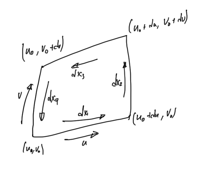
Posted in Math and Physics Learning. | Tagged: , , , , , , , , , , , , , , , , , , , , , , , , , , , , , , , , , , , , | 8 Comments »

Tangent planes and normals in three and four dimensions

Posted by peeterjoot on January 4, 2013

[Click here for a PDF of this post with nicer formatting]

Motivation

I was reviewing the method of Lagrange in my old first year calculus book [1] and found that I needed a review of some of the geometry ideas associated with the gradient (that it is normal to the surface). The approach in the text used 3D level surfaces f(x, y, z) = c, which is general but not the most intuitive.

If we define a surface in the simpler explicit form z = f(x, y), then how would you show this normal property? Here we explore this in 3D and 4D, using geometric and wedge products to express the tangent planes and tangent volumes respectively.

In the 4D approach, with a vector x defined by coordinates x^\mu and basis \{\gamma_\mu\} so that

\begin{aligned}x = \gamma_\mu x^\mu,\end{aligned} \hspace{\stretch{1}}(1.1.1)

the reciprocal basis {\gamma^\mu} is defined implicitly by the dot product relations

\begin{aligned}\gamma^\mu \cdot \gamma_\nu = {\delta^\mu}_\nu.\end{aligned} \hspace{\stretch{1}}(1.1.2)

Assuming such a basis makes the result general enough that the 4D (or a trivial generalization to N dimensions) holds for both Euclidean spaces as well as mixed metric (i.e. Minkowski) spaces, and avoids having to detail the specific metric in question.

3D surface

We start by considering figure 1:

Figure 1: A portion of a surface in 3D


We wish to determine the bivector for the tangent plane in the neighbourhood of the point \mathbf{p}

\begin{aligned}\mathbf{p} = ( x, y, f(x, y) ),\end{aligned} \hspace{\stretch{1}}(1.2.3)

then using duality determine the normal vector to that plane at this point. Holding either of the two free parameters constant, we find the tangent vectors on that surface to be

\begin{aligned}\mathbf{p}_1 = \left( dx, 0, \frac{\partial {f}}{\partial {x}} dx \right) \propto \left( 1, 0, \frac{\partial {f}}{\partial {x}} \right) \end{aligned} \hspace{\stretch{1}}(1.0.4a)

\begin{aligned}\mathbf{p}_2 = \left( 0, dy, \frac{\partial {f}}{\partial {y}} dy \right) \propto \left( 0, 1, \frac{\partial {f}}{\partial {y}} \right) \end{aligned} \hspace{\stretch{1}}(1.0.4b)

The tangent plane is then

\begin{aligned}\mathbf{p}_1 \wedge \mathbf{p}_2 &= \left( 1, 0, \frac{\partial {f}}{\partial {x}} \right) \wedge\left( 0, 1, \frac{\partial {f}}{\partial {y}} \right) \\ &= \left( \mathbf{e}_1 + \mathbf{e}_3 \frac{\partial {f}}{\partial {x}} \right) \wedge\left( \mathbf{e}_2 + \mathbf{e}_3 \frac{\partial {f}}{\partial {y}} \right) \\ &= \mathbf{e}_1 \mathbf{e}_2 + \mathbf{e}_1 \mathbf{e}_3 \frac{\partial {f}}{\partial {y}} + \mathbf{e}_3 \mathbf{e}_2 \frac{\partial {f}}{\partial {x}}.\end{aligned} \hspace{\stretch{1}}(1.0.5)

We can factor out the pseudoscalar 3D volume element I = \mathbf{e}_1 \mathbf{e}_2 \mathbf{e}_3, assuming a Euclidean space for which \mathbf{e}_k^2 = 1. That is

\begin{aligned}\mathbf{p}_1 \wedge \mathbf{p}_2 = \mathbf{e}_1 \mathbf{e}_2 \mathbf{e}_3 \left(\mathbf{e}_3- \mathbf{e}_2 \frac{\partial {f}}{\partial {y}} - \mathbf{e}_1 \frac{\partial {f}}{\partial {x}}\right)\end{aligned} \hspace{\stretch{1}}(1.0.6)

Multiplying through by the volume element I we find that the normal to the surface at this point is

\begin{aligned}\mathbf{n} \propto -I(\mathbf{p}_1 \wedge \mathbf{p}_2) = \mathbf{e}_3- \mathbf{e}_1 \frac{\partial {f}}{\partial {x}}- \mathbf{e}_2 \frac{\partial {f}}{\partial {y}}.\end{aligned} \hspace{\stretch{1}}(1.0.7)

Observe that we can write this as

\begin{aligned}\boxed{\mathbf{n} = \boldsymbol{\nabla} ( z - f(x, y) ).}\end{aligned} \hspace{\stretch{1}}(1.0.8)

Let’s see how this works in 4D, so that we know how to handle the Minkowski spaces we find in special relativity.

4D surface

Now, let’s move up to one additional direction, with

\begin{aligned}x^3 = f(x^0, x^1, x^2).\end{aligned} \hspace{\stretch{1}}(1.0.9)

the differential of this is

\begin{aligned}dx^3 = \sum_{k=0}^2 \frac{\partial {f}}{\partial {x^k}} dx^k = \sum_{k=0}^2 \partial_k f dx^k .\end{aligned} \hspace{\stretch{1}}(1.0.10)

We are going to look at the 3-surface in the neighbourhood of the point

\begin{aligned}p = \left( x^0, x^1, x^2, x^3\right),\end{aligned} \hspace{\stretch{1}}(1.0.11)

so that the tangent vectors in the neighbourhood of this point are in the span of

\begin{aligned}dp = \left( x^0, x^1, x^2, \sum_{k=0}^2 \partial_k dx^k\right).\end{aligned} \hspace{\stretch{1}}(1.0.12)

In particular, in each of the directions we have

\begin{aligned}p_0 \propto ( 1, 0, 0, d_0 f)\end{aligned} \hspace{\stretch{1}}(1.0.13a)

\begin{aligned}p_1 \propto ( 0, 1, 0, d_1 f)\end{aligned} \hspace{\stretch{1}}(1.0.13b)

\begin{aligned}p_2 \propto ( 0, 0, 1, d_2 f)\end{aligned} \hspace{\stretch{1}}(1.0.13c)

Our tangent volume in this neighbourhood is

\begin{aligned}p_0 \wedge p_1 \wedge p_2&=\left( \gamma_0 + \gamma_3 \partial_0 f\right)\wedge\left( \gamma_1 + \gamma_3 \partial_1 f\right)\wedge\left( \gamma_2 + \gamma_3 \partial_2 f\right) \\ &=\left( \gamma_0 \gamma_1 + \gamma_0 \gamma_3 \partial_1 f+ \gamma_3 \gamma_1 \partial_0 f\right)\wedge\left( \gamma_2 + \gamma_3 \partial_2 f\right) \\ &=\gamma_{012} - \gamma_{023} \partial_1 f + \gamma_{123} \partial_0 f + \gamma_{013} \partial_2 f.\end{aligned} \hspace{\stretch{1}}(1.0.14)

Here the shorthand \gamma_{ijk} = \gamma_i \gamma_j \gamma_k has been used. Can we factor out a 4D pseudoscalar from this and end up with a coherent result. We have

\begin{aligned}\gamma_{0123} \gamma^3 = \gamma_{012}\end{aligned} \hspace{\stretch{1}}(1.0.15a)

\begin{aligned}\gamma_{0123} \gamma^1 = \gamma_{023}\end{aligned} \hspace{\stretch{1}}(1.0.15b)

\begin{aligned}\gamma_{0123} \gamma^0 = -\gamma_{123}\end{aligned} \hspace{\stretch{1}}(1.0.15c)

\begin{aligned}\gamma_{0123} \gamma^2 = -\gamma_{013}.\end{aligned} \hspace{\stretch{1}}(1.0.15d)

This gives us

\begin{aligned}d^3 p=p_0 \wedge p_1 \wedge p_2=\gamma_{0123} \left(\gamma^3 - \gamma^1 \partial_1 f- \gamma^0 \partial_0 f- \gamma^2 \partial_2 f\right).\end{aligned} \hspace{\stretch{1}}(1.0.16)

With the usual 4d gradient definition (sum implied)

\begin{aligned}\nabla = \gamma^\mu \partial_\mu,\end{aligned} \hspace{\stretch{1}}(1.0.17)

we have

\begin{aligned}\nabla x^3 = \gamma^\mu \partial_\mu x^3 = \gamma^\mu {\delta_{\mu}}^3= \gamma^3,\end{aligned} \hspace{\stretch{1}}(1.0.18)

so we can write

\begin{aligned}d^3 p = \gamma_{0123} \nabla \left( x^3 - f(x^0, x^1, x^2) \right),\end{aligned} \hspace{\stretch{1}}(1.0.19)

so, finally, the “normal” to this surface volume element at this point is

\begin{aligned}\boxed{n = \nabla \left( x^3 - f(x^0, x^1, x^2) \right).}\end{aligned} \hspace{\stretch{1}}(1.0.20)

This is just like the 3D Euclidean result, with the exception that we need to look at the dual of a 3-volume “surface” instead of our normal 2d surface.

Also note that this is not a metric free result. The metric choice is built into the definition of the gradient 1.0.17 and its associated reciprocal basis. For example with a 1,3 metric where \gamma_0^2 = 1, \gamma_k^2 = -1, we have \gamma^0 = \gamma_0 and \gamma^k = -\gamma_k.

References

[1] S.L. Salas, E. Hille, G.J. Etgen, and G.J. Etgen. Calculus: one and several variables. Wiley New York, 1990.

Posted in Math and Physics Learning. | Tagged: , , , , , , , , , , , | Leave a Comment »

PHY454H1S Continuum Mechanics. Lecture 7: P-waves and S-waves. Taught by Prof. K. Das.

Posted by peeterjoot on February 1, 2012

[Click here for a PDF of this post with nicer formatting and figures if the post had any (especially if my latex to wordpress script has left FORMULA DOES NOT PARSE errors.)]

Disclaimer.

Peeter’s lecture notes from class. May not be entirely coherent.

Setup

Reading: section 22 from [1].

We got as far as expressing the vector displacement \mathbf{e} for an isotropic material at a given point in terms of the Lam\’e parameters

\begin{aligned}\rho \frac{\partial^2 {\mathbf{e}}}{\partial {{t}}^2} = (\lambda + \mu) \boldsymbol{\nabla} (\boldsymbol{\nabla} \cdot \mathbf{e}) + \mu \boldsymbol{\nabla}^2 \mathbf{e}.\end{aligned} \hspace{\stretch{1}}(2.1)

P-waves.

Operating on this with the divergence once more, and writing \theta = \boldsymbol{\nabla} \cdot \mathbf{e}, we have

\begin{aligned}\rho \frac{\partial^2 {{\boldsymbol{\nabla} \cdot \mathbf{e}}}}{\partial {{t}}^2} = (\lambda + \mu) \boldsymbol{\nabla} \cdot \boldsymbol{\nabla} (\boldsymbol{\nabla} \cdot \mathbf{e}) + \mu \boldsymbol{\nabla}^2 (\boldsymbol{\nabla} \cdot \mathbf{e})\end{aligned} \hspace{\stretch{1}}(2.2)

or

\begin{aligned}\frac{\partial^2 {{\theta}}}{\partial {{t}}^2} = \frac{\lambda + 2 \mu}{\rho} \boldsymbol{\nabla}^2 \theta.\end{aligned} \hspace{\stretch{1}}(2.3)

We see that our divergence is governed by a wave equation where the speed of the wave C_L is specified by

\begin{aligned}C_L^2 = \frac{\lambda + 2 \mu}{\rho},\end{aligned} \hspace{\stretch{1}}(2.4)

so the displacement wave equation is given by

\begin{aligned}\frac{\partial^2 {{\theta}}}{\partial {{t}}^2} = C_L^2 \boldsymbol{\nabla}^2 \theta.\end{aligned} \hspace{\stretch{1}}(2.5)

Let’s look at the divergence of the displacement vector in some more detail. By definition this is just

\begin{aligned}\boldsymbol{\nabla} \cdot \mathbf{e} = \frac{\partial {e_1}}{\partial {x_1}}+\frac{\partial {e_2}}{\partial {x_2}}+\frac{\partial {e_3}}{\partial {x_3}}.\end{aligned} \hspace{\stretch{1}}(2.6)

Recall that the strain tensor e_{ij} was defined as

\begin{aligned}e_{ij} = \frac{1}{{2}} \left( \frac{\partial {e_i}}{\partial {x_j}}+\frac{\partial {e_j}}{\partial {x_i}}\right),\end{aligned} \hspace{\stretch{1}}(2.7)

so we have

\begin{aligned}\frac{\partial {e_1}}{\partial {x_1}} &= e_{11} \\ \frac{\partial {e_2}}{\partial {x_2}} &= e_{22} \\ \frac{\partial {e_3}}{\partial {x_3}} &= e_{33}.\end{aligned} \hspace{\stretch{1}}(2.8)

So the divergence in question can be written in terms of the strain tensor

\begin{aligned}\boldsymbol{\nabla} \cdot \mathbf{e} = e_{11}+e_{22}+e_{33} = e_{ii}.\end{aligned} \hspace{\stretch{1}}(2.11)

We also found that the trace of the strain tensor was the relative change in volume. We call this the dilatation. A measure of change in volume as illustrated (badly) in figure (\ref{fig:continuumL7:continuumL7fig1})

\begin{figure}[htp]
\centering
\includegraphics[totalheight=0.2\textheight]{continuumL7fig1}
\caption{Illustrating changes in a control volume.}
\end{figure}

This idea can be found nicely animated in the wikipedia page [2].

S-waves.

Now let’s operate on our equation 2.1 with the curl operator

\begin{aligned}\rho \frac{\partial^2 {{\boldsymbol{\nabla} \times \mathbf{e}}}}{\partial {{t}}^2} = (\lambda + \mu) \boldsymbol{\nabla} \times (\boldsymbol{\nabla} (\boldsymbol{\nabla} \cdot \mathbf{e})) + \mu \boldsymbol{\nabla}^2 (\boldsymbol{\nabla} \times \mathbf{e}).\end{aligned} \hspace{\stretch{1}}(2.12)

Writing

\begin{aligned}\boldsymbol{\omega} = \boldsymbol{\nabla} \times \mathbf{e},\end{aligned} \hspace{\stretch{1}}(2.13)

and observing that \boldsymbol{\nabla} \times \boldsymbol{\nabla} f = 0 (with f = \boldsymbol{\nabla} \cdot \mathbf{e}), we find

\begin{aligned}\rho \frac{\partial^2 {{\boldsymbol{\omega}}}}{\partial {{t}}^2} = \mu \boldsymbol{\nabla}^2 \boldsymbol{\omega}.\end{aligned} \hspace{\stretch{1}}(2.14)

We call this the S-wave equation, and write C_T for the speed of this wave

\begin{aligned}C_T^2 = \mu,\end{aligned} \hspace{\stretch{1}}(2.15)

so that we have

\begin{aligned}\frac{\partial^2 {{\boldsymbol{\omega}}}}{\partial {{t}}^2} = C_T^2 \boldsymbol{\nabla}^2 \boldsymbol{\omega}.\end{aligned} \hspace{\stretch{1}}(2.16)

Again, we can find nice animations of this on wikipedia [3].

Relative speeds of the p-waves and s-waves.

Taking ratios of the wave speeds we find

\begin{aligned}\frac{C_L}{C_T} = \sqrt{\frac{ \lambda + 2 \mu}{\mu}} = \sqrt{ \frac{\lambda}{\mu} + 2}.\end{aligned} \hspace{\stretch{1}}(2.17)

Since both \lambda > 0 and \mu > 0, we have

\begin{aligned}C_L > C_T.\end{aligned} \hspace{\stretch{1}}(2.18)

Divergence (p-waves) are faster than rotational (s-waves) waves.

In terms of the Poisson ratio \nu = \lambda/(2(\lambda + \mu)), we find

\begin{aligned}\frac{\mu}{\lambda} = \frac{1}{{2 \nu}} - 1.\end{aligned} \hspace{\stretch{1}}(2.19)

we see that Poisson’s ratio characterizes the speeds of the waves for the medium

\begin{aligned}\frac{C_L}{C_T} = \sqrt{\frac{2(1-\nu)}{1 - 2\nu}}\end{aligned} \hspace{\stretch{1}}(2.20)

Assuming a gradient plus curl representation.

Let’s assume that our displacement can be written in terms of a gradient and curl as we do for the electric field

\begin{aligned}\mathbf{e} = \boldsymbol{\nabla} \phi + \boldsymbol{\nabla} \times \mathbf{H},\end{aligned} \hspace{\stretch{1}}(2.21)

Inserting this into 2.1 we find

\begin{aligned}\rho \frac{\partial^2 {{(\boldsymbol{\nabla} \phi + \boldsymbol{\nabla} \times \mathbf{H})}}}{\partial {{t}}^2} = (\lambda + \mu) \boldsymbol{\nabla} (\boldsymbol{\nabla} \cdot (\boldsymbol{\nabla} \phi + \boldsymbol{\nabla} \times \mathbf{H})) + \mu \boldsymbol{\nabla}^2 (\boldsymbol{\nabla} \phi + \boldsymbol{\nabla} \times \mathbf{H}).\end{aligned} \hspace{\stretch{1}}(2.22)

using

\begin{aligned}\boldsymbol{\nabla} \cdot \boldsymbol{\nabla} \phi = \boldsymbol{\nabla}^2 \phi.\end{aligned} \hspace{\stretch{1}}(2.23)

Observe that

\begin{aligned}\boldsymbol{\nabla} \cdot (\boldsymbol{\nabla} \times \mathbf{H}) &=\partial_k (\partial_a H_b \epsilon_{abk})&=0\end{aligned}

Here we make use of the fact that an antisymmetric sum of symmetric partials is zero assuming sufficient continuity. Grouping terms we have

\begin{aligned}\boldsymbol{\nabla} \left(\rho \frac{\partial^2 {{\phi}}}{\partial {{t}}^2} - (\lambda + 2\mu) \boldsymbol{\nabla}^2 \phi\right)+ \boldsymbol{\nabla} \times \left(\rho \frac{\partial^2 {\mathbf{H}}}{\partial {{t}}^2} - \mu \boldsymbol{\nabla}^2 \mathbf{H}\right)= 0.\end{aligned} \hspace{\stretch{1}}(2.24)

When the material is infinite in scope, so that boundary value coupling is not a factor, we can write this as a set of independent P-wave and S-wave equations

\begin{aligned}\rho \frac{\partial^2 {{\phi}}}{\partial {{t}}^2} - (\lambda + 2\mu) \boldsymbol{\nabla}^2 \phi = 0\end{aligned} \hspace{\stretch{1}}(2.25)

The P-wave is irrotational (curl free).

\begin{aligned}\rho \frac{\partial^2 {\mathbf{H}}}{\partial {{t}}^2} - \mu \boldsymbol{\nabla}^2 \mathbf{H} = 0\end{aligned} \hspace{\stretch{1}}(2.26)

The S-wave is solenoidal (divergence free).

A couple summarizing statements.

\begin{itemize}
\item
P-waves: irrotational. Volume not preserved.
\item
S-waves: divergence freee. Shearing forces are present and volume is preserved.
\item
P-waves are faster than S-waves.
\end{itemize}

References

[1] L.D. Landau, EM Lifshitz, JB Sykes, WH Reid, and E.H. Dill. Theory of elasticity: Vol. 7 of course of theoretical physics. 1960.

[2] Wikipedia. P-wave — wikipedia, the free encyclopedia [online]. 2012. [Online; accessed 1-February-2012]. http://en.wikipedia.org/w/index.php?title=P-wave&oldid=474119033.

[3] Wikipedia. S-wave — wikipedia, the free encyclopedia [online]. 2011. [Online; accessed 1-February-2012]. http://en.wikipedia.org/w/index.php?title=S-wave&oldid=468110825.

Posted in Math and Physics Learning. | Tagged: , , , , , , , , , | Leave a Comment »

PHY450H1S. Relativistic Electrodynamics Lecture 11 (Taught by Prof. Erich Poppitz). Unpacking Lorentz force equation. Lorentz transformations of the strength tensor, Lorentz field invariants, Bianchi identity, and first half of Maxwell’s.

Posted by peeterjoot on February 24, 2011

[Click here for a PDF of this post with nicer formatting (especially if my latex to wordpress script has left FORMULA DOES NOT PARSE errors.)]

Reading.

Covering chapter 3 material from the text [1].

Covering lecture notes pp. 74-83: Lorentz transformation of the strength tensor (82) [Tuesday, Feb. 8] [extra reading for the mathematically minded: gauge field, strength tensor, and gauge transformations in differential form language, not to be covered in class (83)]

Covering lecture notes pp. 84-102: Lorentz invariants of the electromagnetic field (84-86); Bianchi identity and the first half of Maxwell’s equations (87-90)

Chewing on the four vector form of the Lorentz force equation.

After much effort, we arrived at

\begin{aligned}\frac{d{{(m c u_l) }}}{ds} = \frac{e}{c} \left( \partial_l A_i - \partial_i A_l \right) u^i\end{aligned} \hspace{\stretch{1}}(2.1)

or

\begin{aligned}\frac{d{{ p_l }}}{ds} = \frac{e}{c} F_{l i} u^i\end{aligned} \hspace{\stretch{1}}(2.2)

Elements of the strength tensor

\paragraph{Claim}: there are only 6 independent elements of this matrix (tensor)

\begin{aligned}\begin{bmatrix}0 & . & . & . \\    & 0 & . & . \\    &   & 0 & . \\    &   &   & 0 \\  \end{bmatrix}\end{aligned} \hspace{\stretch{1}}(2.3)

This is a no-brainer, for we just have to mechanically plug in the elements of the field strength tensor

Recall

\begin{aligned}A^i &= (\phi, \mathbf{A}) \\ A_i &= (\phi, -\mathbf{A})\end{aligned} \hspace{\stretch{1}}(2.4)

\begin{aligned}F_{0\alpha} &= \partial_0 A_\alpha - \partial_\alpha A_0  \\ &= -\partial_0 (\mathbf{A})_\alpha - \partial_\alpha \phi  \\ \end{aligned}

\begin{aligned}F_{0\alpha} = E_\alpha\end{aligned} \hspace{\stretch{1}}(2.6)

For the purely spatial index combinations we have

\begin{aligned}F_{\alpha\beta} &= \partial_\alpha A_\beta - \partial_\beta A_\alpha  \\ &= -\partial_\alpha (\mathbf{A})_\beta + \partial_\beta (\mathbf{A})_\alpha  \\ \end{aligned}

Written out explicitly, these are

\begin{aligned}F_{1 2} &= \partial_2 (\mathbf{A})_1 -\partial_1 (\mathbf{A})_2  \\ F_{2 3} &= \partial_3 (\mathbf{A})_2 -\partial_2 (\mathbf{A})_3  \\ F_{3 1} &= \partial_1 (\mathbf{A})_3 -\partial_3 (\mathbf{A})_1 .\end{aligned} \hspace{\stretch{1}}(2.7)

We can compare this to the elements of \mathbf{B}

\begin{aligned}\mathbf{B} = \begin{vmatrix}\hat{\mathbf{x}} & \hat{\mathbf{y}} & \hat{\mathbf{z}} \\ \partial_1 & \partial_2 & \partial_3 \\ A_x & A_y & A_z\end{vmatrix}\end{aligned} \hspace{\stretch{1}}(2.10)

We see that

\begin{aligned}(\mathbf{B})_z &= \partial_1 A_y - \partial_2 A_x \\ (\mathbf{B})_x &= \partial_2 A_z - \partial_3 A_y \\ (\mathbf{B})_y &= \partial_3 A_x - \partial_1 A_z\end{aligned} \hspace{\stretch{1}}(2.11)

So we have

\begin{aligned}F_{1 2} &= - (\mathbf{B})_3 \\ F_{2 3} &= - (\mathbf{B})_1 \\ F_{3 1} &= - (\mathbf{B})_2.\end{aligned} \hspace{\stretch{1}}(2.14)

These can be summarized as simply

\begin{aligned}F_{\alpha\beta} = - \epsilon_{\alpha\beta\gamma} B_\gamma.\end{aligned} \hspace{\stretch{1}}(2.17)

This provides all the info needed to fill in the matrix above

\begin{aligned}{\left\lVert{ F_{i j} }\right\rVert} = \begin{bmatrix}0 & E_x & E_y & E_z \\ -E_x & 0 & -B_z & B_y \\ -E_y & B_z & 0 & -B_x \\ -E_z & -B_y & B_x & 0.\end{bmatrix}.\end{aligned} \hspace{\stretch{1}}(2.18)

Index raising of rank 2 tensor

To raise indexes we compute

\begin{aligned}F^{i j} = g^{i l} g^{j k} F_{l k}.\end{aligned} \hspace{\stretch{1}}(2.19)

Justifying the raising operation.

To justify this consider raising one index at a time by applying the metric tensor to our definition of F_{l k}. That is

\begin{aligned}g^{a l} F_{l k} &=g^{a l} (\partial_l A_k - \partial_k A_l) \\ &=\partial^a A_k - \partial_k A^a.\end{aligned}

Now apply the metric tensor once more

\begin{aligned}g^{b k} g^{a l} F_{l k} &=g^{b k} (\partial^a A_k - \partial_k A^a) \\ &=\partial^a A^b - \partial^b A^a.\end{aligned}

This is, by definition F^{a b}. Since a rank 2 tensor has been defined as an object that transforms like the product of two pairs of coordinates, it makes sense that this particular tensor raises in the same fashion as would a product of two vector coordinates (in this case, it happens to be an antisymmetric product of two vectors, and one of which is an operator, but we have the same idea).

Consider the components of the raised F_{i j} tensor.

\begin{aligned}F^{0\alpha} &= -F_{0\alpha} \\ F^{\alpha\beta} &= F_{\alpha\beta}.\end{aligned} \hspace{\stretch{1}}(2.20)

\begin{aligned}{\left\lVert{ F^{i j} }\right\rVert} = \begin{bmatrix}0 & -E_x & -E_y & -E_z \\ E_x & 0 & -B_z & B_y \\ E_y & B_z & 0 & -B_x \\ E_z & -B_y & B_x & 0\end{bmatrix}.\end{aligned} \hspace{\stretch{1}}(2.22)

Back to chewing on the Lorentz force equation.

\begin{aligned}m c \frac{d{{ u_i }}}{ds} = \frac{e}{c} F_{i j} u^j\end{aligned} \hspace{\stretch{1}}(2.23)

\begin{aligned}u^i &= \gamma \left( 1, \frac{\mathbf{v}}{c} \right) \\ u_i &= \gamma \left( 1, -\frac{\mathbf{v}}{c} \right)\end{aligned} \hspace{\stretch{1}}(2.24)

For the spatial components of the Lorentz force equation we have

\begin{aligned}m c \frac{d{{ u_\alpha }}}{ds} &= \frac{e}{c} F_{\alpha j} u^j \\ &= \frac{e}{c} F_{\alpha 0} u^0+ \frac{e}{c} F_{\alpha \beta} u^\beta \\ &= \frac{e}{c} (-E_{\alpha}) \gamma+ \frac{e}{c} (- \epsilon_{\alpha\beta\gamma} B_\gamma ) \frac{v^\beta}{c} \gamma \end{aligned}

But

\begin{aligned}m c \frac{d{{ u_\alpha }}}{ds} &= -m \frac{d{{(\gamma \mathbf{v}_\alpha)}}}{ds} \\ &= -m \frac{d(\gamma \mathbf{v}_\alpha)}{c \sqrt{1 - \frac{\mathbf{v}^2}{c^2}} dt} \\ &= -\gamma \frac{d(m \gamma \mathbf{v}_\alpha)}{c dt}.\end{aligned}

Canceling the common -\gamma/c terms, and switching to vector notation, we are left with

\begin{aligned}\frac{d( m \gamma \mathbf{v}_\alpha)}{dt} = e \left( E_\alpha + \frac{1}{{c}} (\mathbf{v} \times \mathbf{B})_\alpha \right).\end{aligned} \hspace{\stretch{1}}(2.26)

Now for the energy term. We have

\begin{aligned}m c \frac{d{{u_0}}}{ds} &= \frac{e}{c} F_{0\alpha} u^\alpha \\ &= \frac{e}{c} E_{\alpha} \gamma \frac{v^\alpha}{c} \\ \frac{d{{ m c \gamma }}}{ds} &=\end{aligned}

Putting the final two lines into vector form we have

\begin{aligned}\frac{d{{ (m c^2 \gamma)}}}{dt} = e \mathbf{E} \cdot \mathbf{v},\end{aligned} \hspace{\stretch{1}}(2.27)

or

\begin{aligned}\frac{d{{ \mathcal{E} }}}{dt} = e \mathbf{E} \cdot \mathbf{v}\end{aligned} \hspace{\stretch{1}}(2.28)

Transformation of rank two tensors in matrix and index form.

Transformation of the metric tensor, and some identities.

With

\begin{aligned}\hat{G} = {\left\lVert{ g_{i j} }\right\rVert} = {\left\lVert{ g^{i j} }\right\rVert}\end{aligned} \hspace{\stretch{1}}(3.29)

\paragraph{We claim:}
The rank two tensor \hat{G} transforms in the following sort of sandwich operation, and this leaves it invariant

\begin{aligned}\hat{G} \rightarrow \hat{O} \hat{G} \hat{O}^\text{T} = \hat{G}.\end{aligned} \hspace{\stretch{1}}(3.30)

To demonstrate this let’s consider a transformed vector in coordinate form as follows

\begin{aligned}{x'}^i &= O^{i j} x_j = {O^i}_j x^j \\ {x'}_i &= O_{i j} x^j = {O_i}^j x_j.\end{aligned} \hspace{\stretch{1}}(3.31)

We can thus write the equation in matrix form with

\begin{aligned}X &= {\left\lVert{x^i}\right\rVert} \\ X' &= {\left\lVert{{x'}^i}\right\rVert} \\ \hat{O} &= {\left\lVert{{O^i}_j}\right\rVert} \\ X' &= \hat{O} X\end{aligned} \hspace{\stretch{1}}(3.33)

Our invariant for the vector square, which is required to remain unchanged is

\begin{aligned}{x'}^i {x'}_i &= (O^{i j} x_j)(O_{i k} x^k) \\ &= x^k (O^{i j} O_{i k}) x_j.\end{aligned}

This shows that we have a delta function relationship for the Lorentz transform matrix, when we sum over the first index

\begin{aligned}O^{a i} O_{a j} = {\delta^i}_j.\end{aligned} \hspace{\stretch{1}}(3.37)

It appears we can put 3.37 into matrix form as

\begin{aligned}\hat{G} \hat{O}^\text{T} \hat{G} \hat{O} = I\end{aligned} \hspace{\stretch{1}}(3.38)

Now, if one considers that the transpose of a rotation is an inverse rotation, and the transpose of a boost leaves it unchanged, the transpose of a general Lorentz transformation, a composition of an arbitrary sequence of boosts and rotations, must also be a Lorentz transformation, and must then also leave the norm unchanged. For the transpose of our Lorentz transformation \hat{O} lets write

\begin{aligned}\hat{P} = \hat{O}^\text{T}\end{aligned} \hspace{\stretch{1}}(3.39)

For the action of this on our position vector let’s write

\begin{aligned}{x''}^i &= P^{i j} x_j = O^{j i} x_j \\ {x''}_i &= P_{i j} x^j = O_{j i} x^j\end{aligned} \hspace{\stretch{1}}(3.40)

so that our norm is

\begin{aligned}{x''}^a {x''}_a &= (O_{k a} x^k)(O^{j a} x_j) \\ &= x^k (O_{k a} O^{j a} ) x_j \\ &= x^j x_j \\ \end{aligned}

We must then also have an identity when summing over the second index

\begin{aligned}{\delta_{k}}^j = O_{k a} O^{j a} \end{aligned} \hspace{\stretch{1}}(3.42)

Armed with these facts on the products of O_{i j} and O^{i j} we can now consider the transformation of the metric tensor.

The rule (definition) supplied to us for the transformation of an arbitrary rank two tensor, is that this transforms as its indexes transform individually. Very much as if it was the product of two coordinate vectors and we transform those coordinates separately. Doing so for the metric tensor we have

\begin{aligned}g^{i j} &\rightarrow {O^i}_k g^{k m} {O^j}_m \\ &= ({O^i}_k g^{k m}) {O^j}_m \\ &= O^{i m} {O^j}_m \\ &= O^{i m} (O_{a m} g^{a j}) \\ &= (O^{i m} O_{a m}) g^{a j}\end{aligned}

However, by 3.42, we have O_{a m} O^{i m} = {\delta_a}^i, and we prove that

\begin{aligned}g^{i j} \rightarrow g^{i j}.\end{aligned} \hspace{\stretch{1}}(3.43)

Finally, we wish to put the above transformation in matrix form, look more carefully at the very first line

\begin{aligned}g^{i j}&\rightarrow {O^i}_k g^{k m} {O^j}_m \\ \end{aligned}

which is

\begin{aligned}\hat{G} \rightarrow \hat{O} \hat{G} \hat{O}^\text{T} = \hat{G}\end{aligned} \hspace{\stretch{1}}(3.44)

We see that this particular form of transformation, a sandwich between \hat{O} and \hat{O}^\text{T}, leaves the metric tensor invariant.

Lorentz transformation of the electrodynamic tensor

Having identified a composition of Lorentz transformation matrices, when acting on the metric tensor, leaves it invariant, it is a reasonable question to ask how this form of transformation acts on our electrodynamic tensor F^{i j}?

\paragraph{Claim:} A transformation of the following form is required to maintain the norm of the Lorentz force equation

\begin{aligned}\hat{F} \rightarrow \hat{O} \hat{F} \hat{O}^\text{T} ,\end{aligned} \hspace{\stretch{1}}(3.45)

where \hat{F} = {\left\lVert{F^{i j}}\right\rVert}. Observe that our Lorentz force equation can be written exclusively in upper index quantities as

\begin{aligned}m c \frac{d{{u^i}}}{ds} = \frac{e}{c} F^{i j} g_{j l} u^l\end{aligned} \hspace{\stretch{1}}(3.46)

Because we have a vector on one side of the equation, and it transforms by multiplication with by a Lorentz matrix in SO(1,3)

\begin{aligned}\frac{du^i}{ds} \rightarrow \hat{O} \frac{du^i}{ds} \end{aligned} \hspace{\stretch{1}}(3.47)

The LHS of the Lorentz force equation provides us with one invariant

\begin{aligned}(m c)^2 \frac{d{{u^i}}}{ds} \frac{d{{u_i}}}{ds}\end{aligned} \hspace{\stretch{1}}(3.48)

so the RHS must also provide one

\begin{aligned}\frac{e^2}{c^2} F^{i j} g_{j l} u^lF_{i k} g^{k m} u_m=\frac{e^2}{c^2} F^{i j} u_jF_{i k} u^k.\end{aligned} \hspace{\stretch{1}}(3.49)

Let’s look at the RHS in matrix form. Writing

\begin{aligned}U = {\left\lVert{u^i}\right\rVert},\end{aligned} \hspace{\stretch{1}}(3.50)

we can rewrite the Lorentz force equation as

\begin{aligned}m c \dot{U} = \frac{e}{c} \hat{F} \hat{G} U.\end{aligned} \hspace{\stretch{1}}(3.51)

In this matrix formalism our invariant 3.49 is

\begin{aligned}\frac{e^2}{c^2} (\hat{F} \hat{G} U)^\text{T} G \hat{F} \hat{G} U=\frac{e^2}{c^2} U^\text{T} \hat{G} \hat{F}^\text{T} G \hat{F} \hat{G} U.\end{aligned} \hspace{\stretch{1}}(3.52)

If we compare this to the transformed Lorentz force equation we have

\begin{aligned}m c \hat{O} \dot{U} = \frac{e}{c} \hat{F'} \hat{G} \hat{O} U.\end{aligned} \hspace{\stretch{1}}(3.53)

Our invariant for the transformed equation is

\begin{aligned}\frac{e^2}{c^2} (\hat{F'} \hat{G} \hat{O} U)^\text{T} G \hat{F'} \hat{G} \hat{O} U&=\frac{e^2}{c^2} U^\text{T} \hat{O}^\text{T} \hat{G} \hat{F'}^\text{T} G \hat{F'} \hat{G} \hat{O} U \\ \end{aligned}

Thus the transformed electrodynamic tensor \hat{F}' must satisfy the identity

\begin{aligned}\hat{O}^\text{T} \hat{G} \hat{F'}^\text{T} G \hat{F'} \hat{G} \hat{O} = \hat{G} \hat{F}^\text{T} G \hat{F} \hat{G} \end{aligned} \hspace{\stretch{1}}(3.54)

With the substitution \hat{F}' = \hat{O} \hat{F} \hat{O}^\text{T} the LHS is

\begin{aligned}\hat{O}^\text{T} \hat{G} \hat{F'}^\text{T} \hat{G} \hat{F'} \hat{G} \hat{O} &= \hat{O}^\text{T} \hat{G} ( \hat{O} \hat{F} \hat{O}^\text{T})^\T \hat{G} (\hat{O} \hat{F} \hat{O}^\text{T}) \hat{G} \hat{O}  \\ &= (\hat{O}^\text{T} \hat{G} \hat{O}) \hat{F}^\text{T} (\hat{O}^\text{T} \hat{G} \hat{O}) \hat{F} (\hat{O}^\text{T} \hat{G} \hat{O}) \\ \end{aligned}

We’ve argued that \hat{P} = \hat{O}^\text{T} is also a Lorentz transformation, thus

\begin{aligned}\hat{O}^\text{T} \hat{G} \hat{O}&=\hat{P} \hat{G} \hat{O}^\text{T} \\ &=\hat{G}\end{aligned}

This is enough to make both sides of 3.54 match, verifying that this transformation does provide the invariant properties desired.

Direct computation of the Lorentz transformation of the electrodynamic tensor.

We can construct the transformed field tensor more directly, by simply transforming the coordinates of the four gradient and the four potential directly. That is

\begin{aligned}F^{i j} = \partial^i A^j - \partial^j A^i&\rightarrow {O^i}_a {O^j}_b \left( \partial^a A^b - \partial^b A^a \right) \\ &={O^i}_a F^{a b} {O^j}_b \end{aligned}

By inspection we can see that this can be represented in matrix form as

\begin{aligned}\hat{F} \rightarrow \hat{O} \hat{F} \hat{O}^\text{T}\end{aligned} \hspace{\stretch{1}}(3.55)

Four vector invariants

For three vectors \mathbf{A} and \mathbf{B} invariants are

\begin{aligned}\mathbf{A} \cdot \mathbf{B} = A^\alpha B_\alpha\end{aligned} \hspace{\stretch{1}}(4.56)

For four vectors A^i and B^i invariants are

\begin{aligned}A^i B_i = A^i g_{i j} B^j  \end{aligned} \hspace{\stretch{1}}(4.57)

For F_{i j} what are the invariants? One invariant is

\begin{aligned}g^{i j} F_{i j} = 0,\end{aligned} \hspace{\stretch{1}}(4.58)

but this isn’t interesting since it is uniformly zero (product of symmetric and antisymmetric).

The two invariants are

\begin{aligned}F_{i j}F^{i j}\end{aligned} \hspace{\stretch{1}}(4.59)

and

\begin{aligned}\epsilon^{i j k l} F_{i j}F_{k l}\end{aligned} \hspace{\stretch{1}}(4.60)

where

\begin{aligned}\epsilon^{i j k l} =\left\{\begin{array}{l l}0 & \quad \mbox{if any two indexes coincide} \\ 1 & \quad \mbox{for even permutations of i j k l=0123$ } \\ -1 & \quad \mbox{for odd permutations of $i j k l=0123$ } \\ \end{array}\right.\end{aligned} \hspace{\stretch{1}}(4.61)$

We can show (homework) that

\begin{aligned}F_{i j}F^{i j} \propto \mathbf{E}^2 - \mathbf{B}^2\end{aligned} \hspace{\stretch{1}}(4.62)

\begin{aligned}\epsilon^{i j k l} F_{i j}F_{k l} \propto \mathbf{E} \cdot \mathbf{B}\end{aligned} \hspace{\stretch{1}}(4.63)

This first invariant serves as the action density for the Maxwell field equations.

There’s some useful properties of these invariants. One is that if the fields are perpendicular in one frame, then will be in any other.

From the first, note that if {\left\lvert{\mathbf{E}}\right\rvert} > {\left\lvert{\mathbf{B}}\right\rvert}, the invariant is positive, and must be positive in all frames, or if {\left\lvert{\mathbf{E}}\right\rvert}  {\left\lvert{\mathbf{B}}\right\rvert} in one frame, we can transform to a frame with only \mathbf{E}' component, solve that, and then transform back. Similarly if {\left\lvert{\mathbf{E}}\right\rvert} < {\left\lvert{\mathbf{B}}\right\rvert} in one frame, we can transform to a frame with only \mathbf{B}' component, solve that, and then transform back.

The first half of Maxwell’s equations.

\paragraph{Claim: } The source free portions of Maxwell’s equations are a consequence of the definition of the field tensor alone.

Given

\begin{aligned}F_{i j} = \partial_i A_j - \partial_j A_i,\end{aligned} \hspace{\stretch{1}}(5.64)

where

\begin{aligned}\partial_i = \frac{\partial {}}{\partial {x^i}}\end{aligned} \hspace{\stretch{1}}(5.65)

This alone implies half of Maxwell’s equations. To show this we consider

\begin{aligned}e^{m k i j} \partial_k F_{i j} = 0.\end{aligned} \hspace{\stretch{1}}(5.66)

This is the Bianchi identity. To demonstrate this identity, we’ll have to swap indexes, employ derivative commutation, and then swap indexes once more

\begin{aligned}e^{m k i j} \partial_k F_{i j} &= e^{m k i j} \partial_k (\partial_i A_j - \partial_j A_i) \\ &= 2 e^{m k i j} \partial_k \partial_i A_j \\ &= 2 e^{m k i j} \frac{1}{{2}} \left( \partial_k \partial_i A_j + \partial_i \partial_k A_j \right) \\ &= e^{m k i j} \partial_k \partial_i A_j e^{m i k j} \partial_k \partial_i A_j  \\ &= (e^{m k i j} - e^{m k i j}) \partial_k \partial_i A_j \\ &= 0 \qquad \square\end{aligned}

This is the 4D analogue of

\begin{aligned}\boldsymbol{\nabla} \times (\boldsymbol{\nabla} f) = 0\end{aligned} \hspace{\stretch{1}}(5.67)

i.e.

\begin{aligned}e^{\alpha\beta\gamma} \partial_\beta \partial_\gamma f = 0\end{aligned} \hspace{\stretch{1}}(5.68)

Let’s do this explicitly, starting with

\begin{aligned}{\left\lVert{ F_{i j} }\right\rVert} = \begin{bmatrix}0 & E_x & E_y & E_z \\ -E_x & 0 & -B_z & B_y \\ -E_y & B_z & 0 & -B_x \\ -E_z & -B_y & B_x & 0.\end{bmatrix}\end{aligned} \hspace{\stretch{1}}(5.69)

For the m= 0 case we have

\begin{aligned}\epsilon^{0 k i j} \partial_k F_{i j}&=\epsilon^{\alpha \beta \gamma} \partial_\alpha F_{\beta \gamma} \\ &= \epsilon^{\alpha \beta \gamma} \partial_\alpha (-\epsilon_{\beta \gamma \delta} B_\delta) \\ &= -\epsilon^{\alpha \beta \gamma} \epsilon_{\delta \beta \gamma }\partial_\alpha B_\delta \\ &= - 2 {\delta^\alpha}_\delta \partial_\alpha B_\delta \\ &= - 2 \partial_\alpha B_\alpha \end{aligned}

We must then have

\begin{aligned}\partial_\alpha B_\alpha = 0.\end{aligned} \hspace{\stretch{1}}(5.70)

This is just Gauss’s law for magnetism

\begin{aligned}\boldsymbol{\nabla} \cdot \mathbf{B} = 0.\end{aligned} \hspace{\stretch{1}}(5.71)

Let’s do the spatial portion, for which we have three equations, one for each \alpha of

\begin{aligned}e^{\alpha j k l} \partial_j F_{k l}&=e^{\alpha 0 \beta \gamma} \partial_0 F_{\beta \gamma}+e^{\alpha 0 \gamma \beta} \partial_0 F_{\gamma \beta}+e^{\alpha \beta 0 \gamma} \partial_\beta F_{0 \gamma}+e^{\alpha \beta \gamma 0} \partial_\beta F_{\gamma 0}+e^{\alpha \gamma 0 \beta} \partial_\gamma F_{0 \beta}+e^{\alpha \gamma \beta 0} \partial_\gamma F_{\beta 0} \\ &=2 \left( e^{\alpha 0 \beta \gamma} \partial_0 F_{\beta \gamma}+e^{\alpha \beta 0 \gamma} \partial_\beta F_{0 \gamma}+e^{\alpha \gamma 0 \beta} \partial_\gamma F_{0 \beta}\right) \\ &=2 e^{0 \alpha \beta \gamma} \left(-\partial_0 F_{\beta \gamma}+\partial_\beta F_{0 \gamma}- \partial_\gamma F_{0 \beta}\right)\end{aligned}

This implies

\begin{aligned}0 =-\partial_0 F_{\beta \gamma}+\partial_\beta F_{0 \gamma}- \partial_\gamma F_{0 \beta}\end{aligned} \hspace{\stretch{1}}(5.72)

Referring back to the previous expansions of 2.6 and 2.17, we have

\begin{aligned}0 =\partial_0 \epsilon_{\beta\gamma\mu} B_\mu+\partial_\beta E_\gamma- \partial_\gamma E_{\beta},\end{aligned} \hspace{\stretch{1}}(5.73)

or

\begin{aligned}\frac{1}{{c}} \frac{\partial {B_\alpha}}{\partial {t}} + (\boldsymbol{\nabla} \times \mathbf{E})_\alpha = 0.\end{aligned} \hspace{\stretch{1}}(5.74)

These are just the components of the Maxwell-Faraday equation

\begin{aligned}0 = \frac{1}{{c}} \frac{\partial {\mathbf{B}}}{\partial {t}} + \boldsymbol{\nabla} \times \mathbf{E}.\end{aligned} \hspace{\stretch{1}}(5.75)

Appendix. Some additional index gymnastics.

Transposition of mixed index tensor.

Is the transpose of a mixed index object just a substitution of the free indexes? This wasn’t obvious to me that it would be the case, especially since I’d made an error in some index gymnastics that had me temporarily convinced differently. However, working some examples clears the fog. For example let’s take the transpose of 3.37.

\begin{aligned}{\left\lVert{ {\delta^i}_j }\right\rVert}^\text{T} &= {\left\lVert{ O^{a i} O_{a j} }\right\rVert}^\text{T} \\ &= \left( {\left\lVert{ O^{j i} }\right\rVert} {\left\lVert{ O_{i j} }\right\rVert} \right)^\text{T} \\ &={\left\lVert{ O_{i j} }\right\rVert}^\text{T}{\left\lVert{ O^{j i} }\right\rVert}^\text{T}  \\ &={\left\lVert{ O_{j i} }\right\rVert}{\left\lVert{ O^{i j} }\right\rVert} \\ &={\left\lVert{ O_{a i} O^{a j} }\right\rVert} \\ \end{aligned}

If the transpose of a mixed index tensor just swapped the indexes we would have

\begin{aligned}{\left\lVert{ {\delta^i}_j }\right\rVert}^\text{T} = {\left\lVert{ O_{a i} O^{a j} }\right\rVert} \end{aligned} \hspace{\stretch{1}}(6.76)

From this it does appear that all we have to do is switch the indexes and we will write

\begin{aligned}{\delta^j}_i = O_{a i} O^{a j} \end{aligned} \hspace{\stretch{1}}(6.77)

We can consider a more general operation

\begin{aligned}{\left\lVert{{A^i}_j}\right\rVert}^\text{T}&={\left\lVert{ A^{i m} g_{m j} }\right\rVert}^\text{T} \\ &={\left\lVert{ g_{i j} }\right\rVert}^\text{T}{\left\lVert{ A^{i j} }\right\rVert}^\text{T}  \\ &={\left\lVert{ g_{i j} }\right\rVert}{\left\lVert{ A^{j i} }\right\rVert} \\ &={\left\lVert{ g_{i m} A^{j m} }\right\rVert} \\ &={\left\lVert{ {A^{j}}_i }\right\rVert}\end{aligned}

So we see that we do just have to swap indexes.

Transposition of lower index tensor.

We’ve saw above that we had

\begin{aligned}{\left\lVert{ {A^{i}}_j }\right\rVert}^\text{T} &= {\left\lVert{ {A_{j}}^i }\right\rVert} \\ {\left\lVert{ {A_{i}}^j }\right\rVert}^\text{T} &= {\left\lVert{ {A^{j}}_i }\right\rVert} \end{aligned} \hspace{\stretch{1}}(6.78)

which followed by careful treatment of the transposition in terms of A^{i j} for which we defined a transpose operation. We assumed as well that

\begin{aligned}{\left\lVert{ A_{i j} }\right\rVert}^\text{T} = {\left\lVert{ A_{j i} }\right\rVert}.\end{aligned} \hspace{\stretch{1}}(6.80)

However, this does not have to be assumed, provided that g^{i j} = g_{i j}, and (AB)^\text{T} = B^\text{T} A^\text{T}. We see this by expanding this transposition in products of A^{i j} and \hat{G}

\begin{aligned}{\left\lVert{ A_{i j} }\right\rVert}^\text{T}&= \left( {\left\lVert{g_{i j}}\right\rVert} {\left\lVert{ A^{i j} }\right\rVert} {\left\lVert{g_{i j}}\right\rVert} \right)^\text{T} \\ &= \left( {\left\lVert{g^{i j}}\right\rVert} {\left\lVert{ A^{i j} }\right\rVert} {\left\lVert{g^{i j}}\right\rVert} \right)^\text{T} \\ &= {\left\lVert{g^{i j}}\right\rVert}^\text{T} {\left\lVert{ A^{i j}}\right\rVert}^\text{T} {\left\lVert{g^{i j}}\right\rVert}^\text{T} \\ &= {\left\lVert{g^{i j}}\right\rVert} {\left\lVert{ A^{j i}}\right\rVert} {\left\lVert{g^{i j}}\right\rVert} \\ &= {\left\lVert{g_{i j}}\right\rVert} {\left\lVert{ A^{i j}}\right\rVert} {\left\lVert{g_{i j}}\right\rVert} \\ &= {\left\lVert{ A_{j i}}\right\rVert} \end{aligned}

It would be worthwhile to go through all of this index manipulation stuff and lay it out in a structured axiomatic form. What is the minimal set of assumptions, and how does all of this generalize to non-diagonal metric tensors (even in Euclidean spaces).

Translating the index expression of identity from Lorentz products to matrix form

A verification that the matrix expression 3.38, matches the index expression 3.37 as claimed is worthwhile. It would be easy to guess something similar like \hat{O}^\text{T} \hat{G} \hat{O} \hat{G} is instead the matrix representation. That was in fact my first erroneous attempt to form the matrix equivalent, but is the transpose of 3.38. Either way you get an identity, but the indexes didn’t match.

Since we have g^{i j} = g_{i j} which do we pick to do this verification? This appears to be dictated by requirements to match lower and upper indexes on the summed over index. This is probably clearest by example, so let’s expand the products on the LHS explicitly

\begin{aligned}{\left\lVert{ g^{i j} }\right\rVert} {\left\lVert{ {O^{i}}_j }\right\rVert} ^\text{T}{\left\lVert{ g_{i j} }\right\rVert}{\left\lVert{ {O^{i}}_j }\right\rVert} &=\left( {\left\lVert{ {O^{i}}_j }\right\rVert} {\left\lVert{ g^{i j} }\right\rVert} \right) ^\text{T}{\left\lVert{ g_{i j} }\right\rVert}{\left\lVert{ {O^{i}}_j }\right\rVert}  \\ &=\left( {\left\lVert{ {O^{i}}_k g^{k j} }\right\rVert} \right) ^\text{T}{\left\lVert{ g_{i m} {O^{m}}_j }\right\rVert}  \\ &={\left\lVert{ O^{i j} }\right\rVert} ^\text{T}{\left\lVert{ O_{i j} }\right\rVert}  \\ &={\left\lVert{ O^{j i} }\right\rVert} {\left\lVert{ O_{i j} }\right\rVert}  \\ &={\left\lVert{ O^{k i} O_{k j} }\right\rVert}  \\ \end{aligned}

This matches the {\left\lVert{{\delta^i}_j}\right\rVert} that we have on the RHS, and all is well.

References

[1] L.D. Landau and E.M. Lifshitz. The classical theory of fields. Butterworth-Heinemann, 1980.

Posted in Math and Physics Learning. | Tagged: , , , , , , , , , , , , , , , , , , , , , , | Leave a Comment »

Notes and problems for Desai chapter IV.

Posted by peeterjoot on October 12, 2010

[Click here for a PDF of this post with nicer formatting]

Notes.

Chapter IV notes and problems for [1].

There’s a lot of magic related to the spherical Harmonics in this chapter, with identities pulled out of the Author’s butt. It would be nice to work through that, but need a better reference to work from (or skip ahead to chapter 26 where some of this is apparently derived).

Other stuff pending background derivation and verification are

\begin{itemize}
\item Antisymmetric tensor summation identity.

\begin{aligned}\sum_i \epsilon_{ijk} \epsilon_{iab} = \delta_{ja} \delta_{kb} - \delta_{jb}\delta_{ka}\end{aligned} \hspace{\stretch{1}}(1.1)

This is obviously the coordinate equivalent of the dot product of two bivectors

\begin{aligned}(\mathbf{e}_j \wedge \mathbf{e}_k) \cdot (\mathbf{e}_a \wedge \mathbf{e}_b) &=( (\mathbf{e}_j \wedge \mathbf{e}_k) \cdot \mathbf{e}_a ) \cdot \mathbf{e}_b) =\delta_{ka}\delta_{jb} - \delta_{ja}\delta_{kb}\end{aligned} \hspace{\stretch{1}}(1.2)

We can prove 1.1 by expanding the LHS of 1.2 in coordinates

\begin{aligned}(\mathbf{e}_j \wedge \mathbf{e}_k) \cdot (\mathbf{e}_a \wedge \mathbf{e}_b)&= \sum_{ie} \left\langle{{\epsilon_{ijk} \mathbf{e}_j \mathbf{e}_k \epsilon_{eab} \mathbf{e}_a \mathbf{e}_b}}\right\rangle \\ &=\sum_{ie}\epsilon_{ijk} \epsilon_{eab}\left\langle{{(\mathbf{e}_i \mathbf{e}_i) \mathbf{e}_j \mathbf{e}_k (\mathbf{e}_e \mathbf{e}_e) \mathbf{e}_a \mathbf{e}_b}}\right\rangle \\ &=\sum_{ie}\epsilon_{ijk} \epsilon_{eab}\left\langle{{\mathbf{e}_i \mathbf{e}_e I^2}}\right\rangle \\ &=-\sum_{ie} \epsilon_{ijk} \epsilon_{eab} \delta_{ie} \\ &=-\sum_i\epsilon_{ijk} \epsilon_{iab}\qquad\square\end{aligned}

\item Question on raising and lowering arguments.

How equation (4.240) was arrived at is not clear. In (4.239) he writes

\begin{aligned}\int_0^{2\pi} \int_0^{\pi} d\theta d\phi(L_{-} Y_{lm})^\dagger L_{-} Y_{lm} \sin\theta\end{aligned}

Shouldn’t that Hermitian conjugation be just complex conjugation? if so one would have

\begin{aligned}\int_0^{2\pi} \int_0^{\pi} d\theta d\phi L_{-}^{*} Y_{lm}^{*}L_{-} Y_{lm} \sin\theta\end{aligned}

How does he end up with the L_{-} and the Y_{lm}^{*} interchanged. What justifies this commutation?

A much clearer discussion of this can be found in The operators L_{\pm}, where Dirac notation is used for the normalization discussion.

\item Another question on raising and lowering arguments.

The reasoning leading to (4.238) isn’t clear to me. I fail to see how the L_{-} commutation with \mathbf{L}^2 implies this?

\end{itemize}

Problems

Problem 1.

Statement.

Write down the free particle Schr\”{o}dinger equation for two dimensions in (i) Cartesian and (ii) polar coordinates. Obtain the corresponding wavefunction.

Cartesian case.

For the Cartesian coordinates case we have

\begin{aligned}H = -\frac{\hbar^2}{2m} (\partial_{xx} + \partial_{yy}) = i \hbar \partial_t\end{aligned} \hspace{\stretch{1}}(2.3)

Application of separation of variables with \Psi = XYT gives

\begin{aligned}-\frac{\hbar^2}{2m} \left( \frac{X''}{X} +\frac{Y''}{Y} \right) = i \hbar \frac{T'}{T} = E .\end{aligned} \hspace{\stretch{1}}(2.4)

Immediately, we have the time dependence

\begin{aligned}T \propto e^{-i E t/\hbar},\end{aligned} \hspace{\stretch{1}}(2.5)

with the PDE reduced to

\begin{aligned}\frac{X''}{X} +\frac{Y''}{Y} = - \frac{2m E}{\hbar^2}.\end{aligned} \hspace{\stretch{1}}(2.6)

Introducing separate independent constants

\begin{aligned}\frac{X''}{X} &= a^2 \\ \frac{Y''}{Y} &= b^2 \end{aligned} \hspace{\stretch{1}}(2.7)

provides the pre-normalized wave function and the constraints on the constants

\begin{aligned}\Psi &= C e^{ax}e^{by}e^{-iE t/\hbar} \\ a^2 + b^2 &= -\frac{2 m E}{\hbar^2}.\end{aligned} \hspace{\stretch{1}}(2.9)

Rectangular normalization.

We are now ready to apply normalization constraints. One possibility is a rectangular periodicity requirement.

\begin{aligned}e^{ax} &= e^{a(x + \lambda_x)} \\ e^{ay} &= e^{a(y + \lambda_y)} ,\end{aligned} \hspace{\stretch{1}}(2.11)

or

\begin{aligned}a\lambda_x &= 2 \pi i m \\ a\lambda_y &= 2 \pi i n.\end{aligned} \hspace{\stretch{1}}(2.13)

This provides a more explicit form for the energy expression

\begin{aligned}E_{mn} &= \frac{1}{{2m}} 4 \pi^2 \hbar^2 \left( \frac{m^2}{{\lambda_x}^2}+\frac{n^2}{{\lambda_y}^2}\right).\end{aligned} \hspace{\stretch{1}}(2.15)

We can also add in the area normalization using

\begin{aligned}\left\langle{{\psi}} \vert {{\phi}}\right\rangle &= \int_{x=0}^{\lambda_x} dx\int_{y=0}^{\lambda_x} dy \psi^{*}(x,y) \phi(x,y).\end{aligned} \hspace{\stretch{1}}(2.16)

Our eigenfunctions are now completely specified

\begin{aligned}u_{mn}(x,y,t) &= \frac{1}{{\sqrt{\lambda_x \lambda_y}}}e^{2 \pi i x/\lambda_x}e^{2 \pi i y/\lambda_y}e^{-iE t/\hbar}.\end{aligned} \hspace{\stretch{1}}(2.17)

The interesting thing about this solution is that we can make arbitrary linear combinations

\begin{aligned}f(x,y) = a_{mn} u_{mn}\end{aligned} \hspace{\stretch{1}}(2.18)

and then “solve” for a_{mn}, for an arbitrary f(x,y) by taking inner products

\begin{aligned}a_{mn} = \left\langle{{u_mn}} \vert {{f}}\right\rangle =\int_{x=0}^{\lambda_x} dx \int_{y=0}^{\lambda_x} dy f(x,y) u_mn^{*}(x,y).\end{aligned} \hspace{\stretch{1}}(2.19)

This gives the appearance that any function f(x,y) is a solution, but the equality of 2.18 only applies for functions in the span of this function vector space. The procedure works for arbitrary square integrable functions f(x,y), but the equality really means that the RHS will be the periodic extension of f(x,y).

Infinite space normalization.

An alternate normalization is possible by using the Fourier transform normalization, in which we substitute

\begin{aligned}\frac{2 \pi m }{\lambda_x} &= k_x \\ \frac{2 \pi n }{\lambda_y} &= k_y \end{aligned} \hspace{\stretch{1}}(2.20)

Our inner product is now

\begin{aligned}\left\langle{{\psi}} \vert {{\phi}}\right\rangle &= \int_{-\infty}^{\infty} dx\int_{\infty}^{\infty} dy \psi^{*}(x,y) \phi(x,y).\end{aligned} \hspace{\stretch{1}}(2.22)

And the corresponding normalized wavefunction and associated energy constant E are

\begin{aligned}u_{\mathbf{k}}(x,y,t) &= \frac{1}{{2\pi}}e^{i k_x x}e^{i k_y y}e^{-iE t/\hbar} = \frac{1}{{2\pi}}e^{i \mathbf{k} \cdot \mathbf{x}}e^{-iE t/\hbar} \\ E &= \frac{\hbar^2 \mathbf{k}^2 }{2m}\end{aligned} \hspace{\stretch{1}}(2.23)

Now via this Fourier inner product we are able to construct a solution from any square integrable function. Again, this will not be
an exact equality since the Fourier transform has the effect of averaging across discontinuities.

Polar case.

In polar coordinates our gradient is

\begin{aligned}\boldsymbol{\nabla} &= \hat{\mathbf{r}} \partial_r + \frac{\hat{\boldsymbol{\theta}}}{r} \partial_\theta.\end{aligned} \hspace{\stretch{1}}(2.25)

with

\begin{aligned}\hat{\mathbf{r}} &= \mathbf{e}_1 e^{\mathbf{e}_1 \mathbf{e}_2 \theta} \\ \hat{\boldsymbol{\theta}} &= \mathbf{e}_2 e^{\mathbf{e}_1 \mathbf{e}_2 \theta} .\end{aligned} \hspace{\stretch{1}}(2.26)

Squaring the gradient for the Laplacian we’ll need the partials, which are

\begin{aligned}\partial_r \hat{\mathbf{r}} &= 0 \\ \partial_r \hat{\boldsymbol{\theta}} &= 0 \\ \partial_\theta \hat{\mathbf{r}} &= \hat{\boldsymbol{\theta}} \\ \partial_\theta \hat{\boldsymbol{\theta}} &= -\hat{\mathbf{r}}.\end{aligned}

The Laplacian is therefore

\begin{aligned}\boldsymbol{\nabla}^2 &= (\hat{\mathbf{r}} \partial_r + \frac{\hat{\boldsymbol{\theta}}}{r} \partial_\theta) \cdot(\hat{\mathbf{r}} \partial_r + \frac{\hat{\boldsymbol{\theta}}}{r} \partial_\theta) \\ &= \partial_{rr} + \frac{\hat{\boldsymbol{\theta}}}{r} \cdot \partial_\theta \hat{\mathbf{r}} \partial_r \frac{\hat{\boldsymbol{\theta}}}{r} \cdot \partial_\theta \frac{\hat{\boldsymbol{\theta}}}{r} \partial_\theta \\ &= \partial_{rr} + \frac{\hat{\boldsymbol{\theta}}}{r} \cdot (\partial_\theta \hat{\mathbf{r}}) \partial_r + \frac{\hat{\boldsymbol{\theta}}}{r} \cdot \frac{\hat{\boldsymbol{\theta}}}{r} \partial_{\theta\theta} + \frac{\hat{\boldsymbol{\theta}}}{r} \cdot (\partial_\theta \hat{\boldsymbol{\theta}}) \frac{1}{{r}} \partial_\theta .\end{aligned}

Evalating the derivatives we have

\begin{aligned}\boldsymbol{\nabla}^2 = \partial_{rr} + \frac{1}{{r}} \partial_r + \frac{1}{r^2} \partial_{\theta\theta},\end{aligned} \hspace{\stretch{1}}(2.28)

and are now prepared to move on to the solution of the Hamiltonian H = -(\hbar^2/2m) \boldsymbol{\nabla}^2. With separation of variables again using \Psi = R(r) \Theta(\theta) T(t) we have

\begin{aligned}-\frac{\hbar^2}{2m} \left( \frac{R''}{R} + \frac{R'}{rR} + \frac{1}{{r^2}} \frac{\Theta''}{\Theta} \right) = i \hbar \frac{T'}{T} = E.\end{aligned} \hspace{\stretch{1}}(2.29)

Rearranging to separate the \Theta term we have

\begin{aligned}\frac{r^2 R''}{R} + \frac{r R'}{R} + \frac{2 m E}{\hbar^2} r^2 E = -\frac{\Theta''}{\Theta} = \lambda^2.\end{aligned} \hspace{\stretch{1}}(2.30)

The angular solutions are given by

\begin{aligned}\Theta = \frac{1}{{\sqrt{2\pi}}} e^{i \lambda \theta}\end{aligned} \hspace{\stretch{1}}(2.31)

Where the normalization is given by

\begin{aligned}\left\langle{{\psi}} \vert {{\phi}}\right\rangle &= \int_{0}^{2 \pi} d\theta \psi^{*}(\theta) \phi(\theta).\end{aligned} \hspace{\stretch{1}}(2.32)

And the radial by the solution of the PDE

\begin{aligned}r^2 R'' + r R' + \left( \frac{2 m E}{\hbar^2} r^2 E - \lambda^2 \right) R = 0\end{aligned} \hspace{\stretch{1}}(2.33)

Problem 2.

Statement.

Use the orthogonality property of P_l(\cos\theta)

\begin{aligned}\int_{-1}^1 dx P_l(x) P_{l'}(x) = \frac{2}{2l+1} \delta_{l l'},\end{aligned} \hspace{\stretch{1}}(2.34)

confirm that at least the first two terms of (4.171)

\begin{aligned}e^{i k r \cos\theta} = \sum_{l=0}^\infty (2l + 1) i^l j_l(kr) P_l(\cos\theta)\end{aligned} \hspace{\stretch{1}}(2.35)

are correct.

Solution.

Taking the inner product using the integral of 2.34 we have

\begin{aligned}\int_{-1}^1 dx e^{i k r x} P_l'(x) = 2 i^l j_l(kr) \end{aligned} \hspace{\stretch{1}}(2.36)

To confirm the first two terms we need

\begin{aligned}P_0(x) &= 1 \\ P_1(x) &= x \\ j_0(\rho) &= \frac{\sin\rho}{\rho} \\ j_1(\rho) &= \frac{\sin\rho}{\rho^2} - \frac{\cos\rho}{\rho}.\end{aligned} \hspace{\stretch{1}}(2.37)

On the LHS for l'=0 we have

\begin{aligned}\int_{-1}^1 dx e^{i k r x} = 2 \frac{\sin{kr}}{kr}\end{aligned} \hspace{\stretch{1}}(2.41)

On the LHS for l'=1 note that

\begin{aligned}\int dx x e^{i k r x} &= \int dx x \frac{d}{dx} \frac{e^{i k r x}}{ikr} \\ &= x \frac{e^{i k r x}}{ikr} - \frac{e^{i k r x}}{(ikr)^2}.\end{aligned}

So, integration in [-1,1] gives us

\begin{aligned}\int_{-1}^1 dx e^{i k r x} =  -2i \frac{\cos{kr}}{kr} + 2i \frac{1}{{(kr)^2}} \sin{kr}.\end{aligned} \hspace{\stretch{1}}(2.42)

Now compare to the RHS for l'=0, which is

\begin{aligned}2 j_0(kr) = 2 \frac{\sin{kr}}{kr},\end{aligned} \hspace{\stretch{1}}(2.43)

which matches 2.41. For l'=1 we have

\begin{aligned}2 i j_1(kr) = 2i \frac{1}{{kr}} \left( \frac{\sin{kr}}{kr} - \cos{kr} \right),\end{aligned} \hspace{\stretch{1}}(2.44)

which in turn matches 2.42, completing the exersize.

Problem 3.

Statement.

Obtain the commutation relations \left[{L_i},{L_j}\right] by calculating the vector \mathbf{L} \times \mathbf{L} using the definition \mathbf{L} = \mathbf{r} \times \mathbf{p} directly instead of introducing a differential operator.

Solution.

Expressing the product \mathbf{L} \times \mathbf{L} in determinant form sheds some light on this question. That is

\begin{aligned}\begin{vmatrix} \mathbf{e}_1 & \mathbf{e}_2 & \mathbf{e}_3 \\  L_1 & L_2 & L_3 \\  L_1 & L_2 & L_3\end{vmatrix}&= \mathbf{e}_1 \left[{L_2},{L_3}\right] +\mathbf{e}_2 \left[{L_3},{L_1}\right] +\mathbf{e}_3 \left[{L_1},{L_2}\right]= \mathbf{e}_i \epsilon_{ijk} \left[{L_j},{L_k}\right]\end{aligned} \hspace{\stretch{1}}(2.45)

We see that evaluating this cross product in turn requires evaluation of the set of commutators. We can do that with the canonical commutator relationships directly using L_i = \epsilon_{ijk} r_j p_k like so

\begin{aligned}\left[{L_i},{L_j}\right]&=\epsilon_{imn} r_m p_n \epsilon_{jab} r_a p_b- \epsilon_{jab} r_a p_b \epsilon_{imn} r_m p_n \\ &=\epsilon_{imn} \epsilon_{jab} r_m (p_n r_a) p_b- \epsilon_{jab} \epsilon_{imn} r_a (p_b r_m) p_n \\ &=\epsilon_{imn} \epsilon_{jab} r_m (r_a p_n -i \hbar \delta_{an}) p_b- \epsilon_{jab} \epsilon_{imn} r_a (r_m p_b - i \hbar \delta{mb}) p_n \\ &=\epsilon_{imn} \epsilon_{jab} (r_m r_a p_n p_b - r_a r_m p_b p_n )- i \hbar ( \epsilon_{imn} \epsilon_{jnb} r_m p_b - \epsilon_{jam} \epsilon_{imn} r_a p_n ).\end{aligned}

The first two terms cancel, and we can employ (4.179) to eliminate the antisymmetric tensors from the last two terms

\begin{aligned}\left[{L_i},{L_j}\right]&=i \hbar ( \epsilon_{nim} \epsilon_{njb} r_m p_b - \epsilon_{mja} \epsilon_{min} r_a p_n ) \\ &=i \hbar ( (\delta_{ij} \delta_{mb} -\delta_{ib} \delta_{mj}) r_m p_b - (\delta_{ji} \delta_{an} -\delta_{jn} \delta_{ai}) r_a p_n ) \\ &=i \hbar (\delta_{ij} \delta_{mb} r_m p_b - \delta_{ji} \delta_{an} r_a p_n - \delta_{ib} \delta_{mj} r_m p_b + \delta_{jn} \delta_{ai} r_a p_n ) \\ &=i \hbar (\delta_{ij} r_m p_m- \delta_{ji} r_a p_a- r_j p_i+ r_i p_j ) \\ \end{aligned}

For k \ne i,j, this is i\hbar (\mathbf{r} \times \mathbf{p})_k, so we can write

\begin{aligned}\mathbf{L} \times \mathbf{L} &= i\hbar \mathbf{e}_k \epsilon_{kij} ( r_i p_j - r_j p_i ) = i\hbar \mathbf{L} = i\hbar \mathbf{e}_k L_k = i\hbar \mathbf{L}.\end{aligned} \hspace{\stretch{1}}(2.46)

In [2], the commutator relationships are summarized this way, instead of using the antisymmetric tensor (4.224)

\begin{aligned}\left[{L_i},{L_j}\right] &= i \hbar \epsilon_{ijk} L_k\end{aligned} \hspace{\stretch{1}}(2.47)

as here in Desai. Both say the same thing.

Problem 4.

Statement.

Solution.

TODO.

Problem 5.

Statement.

A free particle is moving along a path of radius R. Express the Hamiltonian in terms of the derivatives involving the polar angle of the particle and write down the Schr\”{o}dinger equation. Determine the wavefunction and the energy eigenvalues of the particle.

Solution.

In classical mechanics our Lagrangian for this system is

\begin{aligned}\mathcal{L} = \frac{1}{{2}} m R^2 \dot{\theta}^2,\end{aligned} \hspace{\stretch{1}}(2.48)

with the canonical momentum

\begin{aligned}p_\theta = \frac{\partial {\mathcal{L}}}{\partial {\dot{\theta}}} = m R^2 \dot{\theta}.\end{aligned} \hspace{\stretch{1}}(2.49)

Thus the classical Hamiltonian is

\begin{aligned}H = \frac{1}{{2m R^2}} {p_\theta}^2.\end{aligned} \hspace{\stretch{1}}(2.50)

By analogy the QM Hamiltonian operator will therefore be

\begin{aligned}H = -\frac{\hbar^2}{2m R^2} \partial_{\theta\theta}.\end{aligned} \hspace{\stretch{1}}(2.51)

For \Psi = \Theta(\theta) T(t), separation of variables gives us

\begin{aligned}-\frac{\hbar^2}{2m R^2} \frac{\Theta''}{\Theta} = i \hbar \frac{T'}{T} = E,\end{aligned} \hspace{\stretch{1}}(2.52)

from which we have

\begin{aligned}T &\propto e^{-i E t/\hbar} \\ \Theta &\propto e^{ \pm i \sqrt{2m E} R \theta/\hbar }.\end{aligned} \hspace{\stretch{1}}(2.53)

Requiring single valued \Theta, equal at any multiples of 2\pi, we have

\begin{aligned}e^{ \pm i \sqrt{2m E} R (\theta + 2\pi)/\hbar } = e^{ \pm i \sqrt{2m E} R \theta/\hbar },\end{aligned}

or

\begin{aligned}\pm \sqrt{2m E} \frac{R}{\hbar} 2\pi = 2 \pi n,\end{aligned}

Suffixing the energy values with this index we have

\begin{aligned}E_n = \frac{n^2 \hbar^2}{2 m R^2}.\end{aligned} \hspace{\stretch{1}}(2.55)

Allowing both positive and negative integer values for n we have

\begin{aligned}\Psi = \frac{1}{{\sqrt{2\pi}}} e^{i n \theta} e^{-i E_n t/\hbar},\end{aligned} \hspace{\stretch{1}}(2.56)

where the normalization was a result of the use of a [0,2\pi] inner product over the angles

\begin{aligned}\left\langle{{\psi}} \vert {{\phi}}\right\rangle \equiv \int_0^{2\pi} \psi^{*}(\theta) \phi(\theta) d\theta.\end{aligned} \hspace{\stretch{1}}(2.57)

Problem 6.

Statement.

Determine \left[{L_i},{r}\right] and \left[{L_i},{\mathbf{r}}\right].

Solution.

Since L_i contain only \theta and \phi partials, \left[{L_i},{r}\right] = 0. For the position vector, however, we have an angular dependence, and are left to evaluate \left[{L_i},{\mathbf{r}}\right] = r \left[{L_i},{\hat{\mathbf{r}}}\right]. We’ll need the partials for \hat{\mathbf{r}}. We have

\begin{aligned}\hat{\mathbf{r}} &= \mathbf{e}_3 e^{I \hat{\boldsymbol{\phi}} \theta} \\ \hat{\boldsymbol{\phi}} &= \mathbf{e}_2 e^{\mathbf{e}_1 \mathbf{e}_2 \phi} \\ I &= \mathbf{e}_1 \mathbf{e}_2 \mathbf{e}_3\end{aligned} \hspace{\stretch{1}}(2.58)

Evaluating the partials we have

\begin{aligned}\partial_\theta \hat{\mathbf{r}} = \hat{\mathbf{r}} I \hat{\boldsymbol{\phi}}\end{aligned}

With

\begin{aligned}\hat{\boldsymbol{\theta}} &= \tilde{R} \mathbf{e}_1 R \\ \hat{\boldsymbol{\phi}} &= \tilde{R} \mathbf{e}_2 R \\ \hat{\mathbf{r}} &= \tilde{R} \mathbf{e}_3 R\end{aligned} \hspace{\stretch{1}}(2.61)

where \tilde{R} R = 1, and \hat{\boldsymbol{\theta}} \hat{\boldsymbol{\phi}} \hat{\mathbf{r}} = \mathbf{e}_1 \mathbf{e}_2 \mathbf{e}_3, we have

\begin{aligned}\partial_\theta \hat{\mathbf{r}} &= \tilde{R} \mathbf{e}_3 \mathbf{e}_1 \mathbf{e}_2 \mathbf{e}_3 \mathbf{e}_2 R = \tilde{R} \mathbf{e}_1 R = \hat{\boldsymbol{\theta}}\end{aligned} \hspace{\stretch{1}}(2.64)

For the \phi partial we have

\begin{aligned}\partial_\phi \hat{\mathbf{r}}&= \mathbf{e}_3 \sin\theta I \hat{\boldsymbol{\phi}} \mathbf{e}_1 \mathbf{e}_2 \\ &= \sin\theta \hat{\boldsymbol{\phi}}\end{aligned}

We are now prepared to evaluate the commutators. Starting with the easiest we have

\begin{aligned}\left[{L_z},{\hat{\mathbf{r}}}\right] \Psi&=-i \hbar (\partial_\phi \hat{\mathbf{r}} \Psi - \hat{\mathbf{r}} \partial_\phi \Psi ) \\ &=-i \hbar (\partial_\phi \hat{\mathbf{r}}) \Psi  \\ \end{aligned}

So we have

\begin{aligned}\left[{L_z},{\hat{\mathbf{r}}}\right]&=-i \hbar \sin\theta \hat{\boldsymbol{\phi}}\end{aligned} \hspace{\stretch{1}}(2.65)

Observe that by virtue of chain rule, only the action of the partials on \hat{\mathbf{r}} itself contributes, and all the partials applied to \Psi cancel out due to the commutator differences. That simplifies the remaining commutator evaluations. For reference the polar form of L_x, and L_y are

\begin{aligned}L_x &= -i \hbar (-S_\phi \partial_\theta - C_\phi \cot\theta \partial_\phi) \\ L_y &= -i \hbar (C_\phi \partial_\theta - S_\phi \cot\theta \partial_\phi),\end{aligned} \hspace{\stretch{1}}(2.66)

where the sines and cosines are written with S, and C respectively for short.

We therefore have

\begin{aligned}\left[{L_x},{\hat{\mathbf{r}}}\right]&= -i \hbar (-S_\phi (\partial_\theta \hat{\mathbf{r}}) - C_\phi \cot\theta (\partial_\phi \hat{\mathbf{r}}) ) \\ &= -i \hbar (-S_\phi \hat{\boldsymbol{\theta}} - C_\phi \cot\theta S_\theta \hat{\boldsymbol{\phi}} ) \\ &= -i \hbar (-S_\phi \hat{\boldsymbol{\theta}} - C_\phi C_\theta \hat{\boldsymbol{\phi}} ) \\ \end{aligned}

and

\begin{aligned}\left[{L_y},{\hat{\mathbf{r}}}\right]&= -i \hbar (C_\phi (\partial_\theta \hat{\mathbf{r}}) - S_\phi \cot\theta (\partial_\phi \hat{\mathbf{r}})) \\ &= -i \hbar (C_\phi \hat{\boldsymbol{\theta}} - S_\phi C_\theta \hat{\boldsymbol{\phi}} ).\end{aligned}

Adding back in the factor of r, and summarizing we have

\begin{aligned}\left[{L_i},{r}\right] &= 0 \\ \left[{L_x},{\mathbf{r}}\right] &= -i \hbar r (-\sin\phi \hat{\boldsymbol{\theta}} - \cos\phi \cos\theta \hat{\boldsymbol{\phi}} ) \\ \left[{L_y},{\mathbf{r}}\right] &= -i \hbar r (\cos\phi \hat{\boldsymbol{\theta}} - \sin\phi \cos\theta \hat{\boldsymbol{\phi}} ) \\ \left[{L_z},{\mathbf{r}}\right] &= -i \hbar r \sin\theta \hat{\boldsymbol{\phi}}\end{aligned} \hspace{\stretch{1}}(2.68)

Problem 7.

Statement.

Show that

\begin{aligned}e^{-i\pi L_x /\hbar } {\lvert {l,m} \rangle} = {\lvert {l,m-1} \rangle}\end{aligned} \hspace{\stretch{1}}(2.72)

Solution.

TODO.

References

[1] BR Desai. Quantum mechanics with basic field theory. Cambridge University Press, 2009.

[2] R. Liboff. Introductory quantum mechanics. 2003.

Posted in Math and Physics Learning. | Tagged: , , , , , , , , , , , , , , , , , , | Leave a Comment »

Derivation of the spherical polar Laplacian

Posted by peeterjoot on October 9, 2010

[Click here for a PDF of this post with nicer formatting]

Motivation.

In [1] was a Geometric Algebra derivation of the 2D polar Laplacian by squaring the quadient. In [2] was a factorization of the spherical polar unit vectors in a tidy compact form. Here both these ideas are utilized to derive the spherical polar form for the Laplacian, an operation that is strictly algebraic (squaring the gradient) provided we operate on the unit vectors correctly.

Our rotation multivector.

Our starting point is a pair of rotations. We rotate first in the x,y plane by \phi

\begin{aligned}\mathbf{x} &\rightarrow \mathbf{x}' = \tilde{R_\phi} \mathbf{x} R_\phi \\ i &\equiv \mathbf{e}_1 \mathbf{e}_2 \\ R_\phi &= e^{i \phi/2}\end{aligned} \hspace{\stretch{1}}(2.1)

Then apply a rotation in the \mathbf{e}_3 \wedge (\tilde{R_\phi} \mathbf{e}_1 R_\phi) = \tilde{R_\phi} \mathbf{e}_3 \mathbf{e}_1 R_\phi plane

\begin{aligned}\mathbf{x}' &\rightarrow \mathbf{x}'' = \tilde{R_\theta} \mathbf{x}' R_\theta \\ R_\theta &= e^{ \tilde{R_\phi} \mathbf{e}_3 \mathbf{e}_1 R_\phi \theta/2 } = \tilde{R_\phi} e^{ \mathbf{e}_3 \mathbf{e}_1 \theta/2 } R_\phi\end{aligned} \hspace{\stretch{1}}(2.4)

The composition of rotations now gives us

\begin{aligned}\mathbf{x}&\rightarrow \mathbf{x}'' = \tilde{R_\theta} \tilde{R_\phi} \mathbf{x} R_\phi R_\theta = \tilde{R} \mathbf{x} R \\ R &= R_\phi R_\theta = e^{ \mathbf{e}_3 \mathbf{e}_1 \theta/2 } e^{ \mathbf{e}_1 \mathbf{e}_2 \phi/2 }.\end{aligned}

Expressions for the unit vectors.

The unit vectors in the rotated frame can now be calculated. With I = \mathbf{e}_1 \mathbf{e}_2 \mathbf{e}_3 we can calculate

\begin{aligned}\hat{\boldsymbol{\phi}} &= \tilde{R} \mathbf{e}_2 R  \\ \hat{\mathbf{r}} &= \tilde{R} \mathbf{e}_3 R  \\ \hat{\boldsymbol{\theta}} &= \tilde{R} \mathbf{e}_1 R\end{aligned} \hspace{\stretch{1}}(3.6)

Performing these we get

\begin{aligned}\hat{\boldsymbol{\phi}}&= e^{ -\mathbf{e}_1 \mathbf{e}_2 \phi/2 } e^{ -\mathbf{e}_3 \mathbf{e}_1 \theta/2 } \mathbf{e}_2 e^{ \mathbf{e}_3 \mathbf{e}_1 \theta/2 } e^{ \mathbf{e}_1 \mathbf{e}_2 \phi/2 } \\ &= \mathbf{e}_2 e^{ i \phi },\end{aligned}

and

\begin{aligned}\hat{\mathbf{r}}&= e^{ -\mathbf{e}_1 \mathbf{e}_2 \phi/2 } e^{ -\mathbf{e}_3 \mathbf{e}_1 \theta/2 } \mathbf{e}_3 e^{ \mathbf{e}_3 \mathbf{e}_1 \theta/2 } e^{ \mathbf{e}_1 \mathbf{e}_2 \phi/2 } \\ &= e^{ -\mathbf{e}_1 \mathbf{e}_2 \phi/2 } (\mathbf{e}_3 \cos\theta + \mathbf{e}_1 \sin\theta ) e^{ \mathbf{e}_1 \mathbf{e}_2 \phi/2 } \\ &= \mathbf{e}_3 \cos\theta +\mathbf{e}_1 \sin\theta e^{ \mathbf{e}_1 \mathbf{e}_2 \phi } \\ &= \mathbf{e}_3 (\cos\theta + \mathbf{e}_3 \mathbf{e}_1 \sin\theta e^{ \mathbf{e}_1 \mathbf{e}_2 \phi } ) \\ &= \mathbf{e}_3 e^{I \hat{\boldsymbol{\phi}} \theta},\end{aligned}

and

\begin{aligned}\hat{\boldsymbol{\theta}}&= e^{ -\mathbf{e}_1 \mathbf{e}_2 \phi/2 } e^{ -\mathbf{e}_3 \mathbf{e}_1 \theta/2 } \mathbf{e}_1 e^{ \mathbf{e}_3 \mathbf{e}_1 \theta/2 } e^{ \mathbf{e}_1 \mathbf{e}_2 \phi/2 } \\ &= e^{ -\mathbf{e}_1 \mathbf{e}_2 \phi/2 } ( \mathbf{e}_1 \cos\theta - \mathbf{e}_3 \sin\theta ) e^{ \mathbf{e}_1 \mathbf{e}_2 \phi/2 } \\ &= \mathbf{e}_1 \cos\theta e^{ \mathbf{e}_1 \mathbf{e}_2 \phi/2 } - \mathbf{e}_3 \sin\theta \\ &= i \hat{\boldsymbol{\phi}} \cos\theta - \mathbf{e}_3 \sin\theta \\ &= i \hat{\boldsymbol{\phi}} (\cos\theta + \hat{\boldsymbol{\phi}} i \mathbf{e}_3 \sin\theta ) \\ &= i \hat{\boldsymbol{\phi}} e^{I \hat{\boldsymbol{\phi}} \theta}.\end{aligned}

Summarizing these are

\begin{aligned}\hat{\boldsymbol{\phi}} &= \mathbf{e}_2 e^{ i \phi } \\ \hat{\mathbf{r}} &= \mathbf{e}_3 e^{I \hat{\boldsymbol{\phi}} \theta} \\ \hat{\boldsymbol{\theta}} &= i \hat{\boldsymbol{\phi}} e^{I \hat{\boldsymbol{\phi}} \theta}.\end{aligned} \hspace{\stretch{1}}(3.9)

Derivatives of the unit vectors.

We’ll need the partials. Most of these can be computed from 3.9 by inspection, and are

\begin{aligned}\partial_r \hat{\boldsymbol{\phi}} &= 0 \\ \partial_r \hat{\mathbf{r}} &= 0 \\ \partial_r \hat{\boldsymbol{\theta}} &= 0 \\ \partial_\theta \hat{\boldsymbol{\phi}} &= 0 \\ \partial_\theta \hat{\mathbf{r}} &= \hat{\mathbf{r}} I \hat{\boldsymbol{\phi}} \\ \partial_\theta \hat{\boldsymbol{\theta}} &= \hat{\boldsymbol{\theta}} I \hat{\boldsymbol{\phi}} \\ \partial_\phi \hat{\boldsymbol{\phi}} &= \hat{\boldsymbol{\phi}} i \\ \partial_\phi \hat{\mathbf{r}} &= \hat{\boldsymbol{\phi}} \sin\theta \\ \partial_\phi \hat{\boldsymbol{\theta}} &= \hat{\boldsymbol{\phi}} \cos\theta\end{aligned} \hspace{\stretch{1}}(4.12)

Expanding the Laplacian.

We note that the line element is ds = dr + r d\theta + r\sin\theta d\phi, so our gradient in spherical coordinates is

\begin{aligned}\boldsymbol{\nabla} &= \hat{\mathbf{r}} \partial_r + \frac{\hat{\boldsymbol{\theta}}}{r} \partial_\theta + \frac{\hat{\boldsymbol{\phi}}}{r\sin\theta} \partial_\phi.\end{aligned} \hspace{\stretch{1}}(5.21)

We can now evaluate the Laplacian

\begin{aligned}\boldsymbol{\nabla}^2 &=\left( \hat{\mathbf{r}} \partial_r + \frac{\hat{\boldsymbol{\theta}}}{r} \partial_\theta + \frac{\hat{\boldsymbol{\phi}}}{r\sin\theta} \partial_\phi \right) \cdot\left( \hat{\mathbf{r}} \partial_r + \frac{\hat{\boldsymbol{\theta}}}{r} \partial_\theta + \frac{\hat{\boldsymbol{\phi}}}{r\sin\theta} \partial_\phi \right).\end{aligned} \hspace{\stretch{1}}(5.22)

Evaluating these one set at a time we have

\begin{aligned}\hat{\mathbf{r}} \partial_r \cdot \left( \hat{\mathbf{r}} \partial_r + \frac{\hat{\boldsymbol{\theta}}}{r} \partial_\theta + \frac{\hat{\boldsymbol{\phi}}}{r\sin\theta} \partial_\phi \right) &= \partial_{rr},\end{aligned}

and

\begin{aligned}\frac{1}{{r}} \hat{\boldsymbol{\theta}} \partial_\theta \cdot \left( \hat{\mathbf{r}} \partial_r + \frac{\hat{\boldsymbol{\theta}}}{r} \partial_\theta + \frac{\hat{\boldsymbol{\phi}}}{r\sin\theta} \partial_\phi \right)&=\frac{1}{{r}} \left\langle{{\hat{\boldsymbol{\theta}} \left(\hat{\mathbf{r}} I \hat{\boldsymbol{\phi}} \partial_r + \hat{\mathbf{r}} \partial_{\theta r}+ \frac{\hat{\boldsymbol{\theta}}}{r} \partial_{\theta\theta} + \frac{1}{{r}} \hat{\boldsymbol{\theta}} I \hat{\boldsymbol{\phi}} \partial_\theta+ \hat{\boldsymbol{\phi}} \partial_\theta \frac{1}{{r\sin\theta}} \partial_\phi\right)}}\right\rangle \\ &= \frac{1}{{r}} \partial_r+\frac{1}{{r^2}} \partial_{\theta\theta},\end{aligned}

and

\begin{aligned}\frac{\hat{\boldsymbol{\phi}}}{r\sin\theta} \partial_\phi &\cdot\left( \hat{\mathbf{r}} \partial_r + \frac{\hat{\boldsymbol{\theta}}}{r} \partial_\theta + \frac{\hat{\boldsymbol{\phi}}}{r\sin\theta} \partial_\phi \right) \\ &=\frac{1}{r\sin\theta} \left\langle{{\hat{\boldsymbol{\phi}}\left(\hat{\boldsymbol{\phi}} \sin\theta \partial_r + \hat{\mathbf{r}} \partial_{\phi r} + \hat{\boldsymbol{\phi}} \cos\theta \frac{1}{r} \partial_\theta + \frac{\hat{\boldsymbol{\theta}}}{r} \partial_{\phi \theta }+ \hat{\boldsymbol{\phi}} i \frac{1}{r\sin\theta} \partial_\phi + \hat{\boldsymbol{\phi}} \frac{1}{r\sin\theta} \partial_{\phi \phi }\right)}}\right\rangle \\ &=\frac{1}{{r}} \partial_r+ \frac{\cot\theta}{r^2}\partial_\theta+ \frac{1}{{r^2 \sin^2\theta}} \partial_{\phi\phi}\end{aligned}

Summing these we have

\begin{aligned}\boldsymbol{\nabla}^2 &=\partial_{rr}+ \frac{2}{r} \partial_r+\frac{1}{{r^2}} \partial_{\theta\theta}+ \frac{\cot\theta}{r^2}\partial_\theta+ \frac{1}{{r^2 \sin^2\theta}} \partial_{\phi\phi}\end{aligned} \hspace{\stretch{1}}(5.23)

This is often written with a chain rule trick to considate the r and \theta partials

\begin{aligned}\boldsymbol{\nabla}^2 \Psi &=\frac{1}{{r}} \partial_{rr} (r \Psi)+ \frac{1}{{r^2 \sin\theta}} \partial_\theta \left( \sin\theta \partial_\theta \Psi \right)+ \frac{1}{{r^2 \sin^2\theta}} \partial_{\psi\psi} \Psi\end{aligned} \hspace{\stretch{1}}(5.24)

It’s simple to verify that this is identical to 5.23.

References

[1] Peeter Joot. Polar form for the gradient and Laplacian. [online]. http://sites.google.com/site/peeterjoot/math2009/polarGradAndLaplacian.pdf.

[2] Peeter Joot. Spherical Polar unit vectors in exponential form. [online]. http://sites.google.com/site/peeterjoot/math2009/sphericalPolarUnit.pdf .

Posted in Math and Physics Learning. | Tagged: , , , , , , , , , | Leave a Comment »

Jacobians and spherical polar gradient

Posted by peeterjoot on December 8, 2009

[Click here for a PDF of this post with nicer formatting]

Motivation

The dumbest and most obvious way to do a chain of variables for the gradient is to utilize a chain rule expansion producing the Jacobian matrix to transform the coordinates. Here we do this to calculate the spherical polar representation of the gradient.

There are smarter and easier ways to do this, but there is some surprising simple structure to the resulting Jacobians that seems worth noting.

Spherical polar gradient coordinates in terms of Cartesian.

We wish to do a change of variables for each of the differential operators of the gradient. This is essentially just application of the chain rule, as in

\begin{aligned}\frac{\partial {}}{\partial {r}} = \frac{\partial {x}}{\partial {r}} \frac{\partial {}}{\partial {x}}+\frac{\partial {y}}{\partial {r}} \frac{\partial {}}{\partial {y}}+\frac{\partial {z}}{\partial {r}} \frac{\partial {}}{\partial {z}}.\end{aligned} \quad\quad\quad(1)

Collecting all such derivatives we have in column vector form

\begin{aligned}\begin{bmatrix}\partial_r \\ \partial_\theta \\ \partial_\phi\end{bmatrix}= \begin{bmatrix}\frac{\partial {x}}{\partial {r}} &\frac{\partial {y}}{\partial {r}} &\frac{\partial {z}}{\partial {r}}  \\ \frac{\partial {x}}{\partial {\theta}} &\frac{\partial {y}}{\partial {\theta}} &\frac{\partial {z}}{\partial {\theta}}  \\ \frac{\partial {x}}{\partial {\phi}} &\frac{\partial {y}}{\partial {\phi}} &\frac{\partial {z}}{\partial {\phi}} \end{bmatrix}\begin{bmatrix}\partial_x \\ \partial_y \\ \partial_z\end{bmatrix}.\end{aligned} \quad\quad\quad(2)

This becomes a bit more tractable with the Jacobian notation

\begin{aligned}\frac{\partial (x,y,z)}{\partial (r,\theta,\phi)}=\begin{bmatrix}\frac{\partial {x}}{\partial {r}} &\frac{\partial {y}}{\partial {r}} &\frac{\partial {z}}{\partial {r}}  \\ \frac{\partial {x}}{\partial {\theta}} &\frac{\partial {y}}{\partial {\theta}} &\frac{\partial {z}}{\partial {\theta}}  \\ \frac{\partial {x}}{\partial {\phi}} &\frac{\partial {y}}{\partial {\phi}} &\frac{\partial {z}}{\partial {\phi}}\end{bmatrix}.\end{aligned} \quad\quad\quad(3)

The change of variables for the operator triplet is then just

\begin{aligned}\begin{bmatrix}\partial_r \\ \partial_\theta \\ \partial_\phi\end{bmatrix}= \frac{\partial (x,y,z)}{\partial (r,\theta,\phi)}\begin{bmatrix}\partial_x \\ \partial_y \\ \partial_z\end{bmatrix}.\end{aligned} \quad\quad\quad(4)

This Jacobian matrix is also not even too hard to calculate. With \mathbf{x} = r \hat{\mathbf{r}}, we have x_k = r \hat{\mathbf{r}} \cdot \mathbf{e}_k, and

\begin{aligned}\frac{\partial {x_k}}{\partial {r}} &= \hat{\mathbf{r}} \cdot \mathbf{e}_k \\ \frac{\partial {x_k}}{\partial {\theta}} &= r \frac{\partial {\hat{\mathbf{r}}}}{\partial {\theta}} \cdot \mathbf{e}_k \\ \frac{\partial {x_k}}{\partial {\phi}} &= r \frac{\partial {\hat{\mathbf{r}}}}{\partial {\phi}} \cdot \mathbf{e}_k.\end{aligned} \quad\quad\quad(5)

The last two derivatives can be calculated easily if the radial unit vector is written out explicitly, with S and C for sine and cosine respectively, these are

\begin{aligned}\hat{\mathbf{r}} &= \begin{bmatrix}S_\theta C_\phi \\ S_\theta S_\phi \\ C_\theta \end{bmatrix} \\ \frac{\partial {\hat{\mathbf{r}}}}{\partial {\theta}} &= \begin{bmatrix}C_\theta C_\phi \\ C_\theta S_\phi \\ -S_\theta \end{bmatrix} \\ \frac{\partial {\hat{\mathbf{r}}}}{\partial {\phi}} &= \begin{bmatrix}-S_\theta S_\phi \\ S_\theta C_\phi \\ 0\end{bmatrix} .\end{aligned} \quad\quad\quad(8)

We can plug these into the elements of the Jacobian matrix explicitly, which produces

\begin{aligned}\frac{\partial (x,y,z)}{\partial (r,\theta,\phi)}=\begin{bmatrix} S_\theta C_\phi & S_\theta S_\phi & C_\theta \\ r C_\theta C_\phi & r C_\theta S_\phi & - r S_\theta \\ -r S_\theta S_\phi & rS_\theta C_\phi & 0\end{bmatrix},\end{aligned} \quad\quad\quad(11)

however, we are probably better off just referring back to 8, and writing

\begin{aligned}\frac{\partial (x,y,z)}{\partial (r,\theta,\phi)}=\begin{bmatrix} \hat{\mathbf{r}}^\text{T} \\ r \frac{\partial {\hat{\mathbf{r}}^\text{T}}}{\partial {\theta}} \\ r \frac{\partial {\hat{\mathbf{r}}^\text{T}}}{\partial {\phi}} \end{bmatrix}.\end{aligned} \quad\quad\quad(12)

Unfortunately, this is actually a bit of a dead end. We really want the inverse of this matrix because the desired quantity is

\begin{aligned}\boldsymbol{\nabla} = \begin{bmatrix}\mathbf{e}_1 & \mathbf{e}_2 & \mathbf{e}_3  \end{bmatrix}\begin{bmatrix}\partial_{x_1} \\ \partial_{x_2} \\ \partial_{x_3}\end{bmatrix}.\end{aligned} \quad\quad\quad(13)

(Here my matrix of unit vectors treats these abusively as single elements and not as column vectors).

The matrix of equation 12 does not look particularly fun to invert directly, and that is what we need to substitute into
13. One knows that in the end if it was attempted things should mystically simplify (presuming this was done error free).

Cartesian gradient coordinates in terms of spherical polar partials.

Let’s flip things upside down and calculate the inverse Jacobian matrix directly. This is a messier job, but it appears less messy than the matrix inversion above.

\begin{aligned}r^2 &= x^2 + y^2 + z^2  \\ \sin^2 \theta &= \frac{x^2 + y^2}{x^2 + y^2 + z^2} \\ \tan\phi &= \frac{y}{x}.\end{aligned} \quad\quad\quad(14)

The messy task is now the calculation of these derivatives.

For the first, from r^2 = x^2 + y^2 + z^2, taking partials on both sides, we have

\begin{aligned}\frac{\partial {r}}{\partial {x_k}} = \frac{x_k}{r}.\end{aligned} \quad\quad\quad(17)

But these are just the direction cosines, the components of our polar unit vector \hat{\mathbf{r}}. We can then write for all of these derivatives in column matrix form

\begin{aligned}\boldsymbol{\nabla} r = \hat{\mathbf{r}}\end{aligned} \quad\quad\quad(18)

Next from \sin^2\theta = (x^2 + y^2)/r^2, we get after some reduction

\begin{aligned}\frac{\partial {\theta}}{\partial {x}} &= \frac{1}{{r}} C_\theta C_\phi \\ \frac{\partial {\phi}}{\partial {y}} &= \frac{1}{{r}} C_\theta S_\phi \\ \frac{\partial {\phi}}{\partial {z}} &= -\frac{S_\theta}{r}.\end{aligned} \quad\quad\quad(19)

Observe that we can antidifferentiate with respect to theta and obtain

\begin{aligned}\boldsymbol{\nabla} \theta &= \frac{1}{{r}}\begin{bmatrix}C_\theta C_\phi \\ C_\theta S_\phi \\ -S_\theta\end{bmatrix} \\ &=\frac{1}{{r}}\frac{\partial {}}{\partial {\theta}}\begin{bmatrix}S_\theta C_\phi \\ S_\theta S_\phi \\ C_\theta\end{bmatrix}.\end{aligned}

This last column vector is our friend the unit polar vector again, and we have

\begin{aligned}\boldsymbol{\nabla} \theta &= \frac{1}{{r}}\frac{\partial {\hat{\mathbf{r}}}}{\partial {\theta}}\end{aligned} \quad\quad\quad(22)

Finally for the \phi dependence we have after some reduction

\begin{aligned}\boldsymbol{\nabla} \phi &=\frac{1}{{r S_\theta}}\begin{bmatrix}-S_\phi \\ C_\phi \\ 0\end{bmatrix}.\end{aligned} \quad\quad\quad(23)

Again, we can antidifferentiate

\begin{aligned}\boldsymbol{\nabla} \phi &=\frac{1}{{r (S_\theta)^2}}\begin{bmatrix}-S_\theta S_\phi \\ S_\theta C_\phi \\ 0\end{bmatrix} \\ &=\frac{1}{{r (S_\theta)^2}}\frac{\partial {}}{\partial {\phi}}\begin{bmatrix}S_\theta C_\phi \\ S_\theta S_\phi \\ C_\theta\end{bmatrix}.\end{aligned}

We have our unit polar vector again, and our \phi partials nicely summarized by

\begin{aligned}\boldsymbol{\nabla} \phi &=\frac{1}{{r (S_\theta)^2}}\frac{\partial {\hat{\mathbf{r}}}}{\partial {\phi}}.\end{aligned} \quad\quad\quad(24)

With this we can now write out the Jacobian matrix either explicitly, or in column vector form in terms of \hat{\mathbf{r}}. First a reminder of why we want this matrix, for the following change of variables

\begin{aligned}\begin{bmatrix}\partial_x \\ \partial_y \\ \partial_z\end{bmatrix}= \begin{bmatrix}\frac{\partial {r}}{\partial {x}} &\frac{\partial {\theta}}{\partial {x}} &\frac{\partial {\phi}}{\partial {x}}  \\ \frac{\partial {r}}{\partial {y}} &\frac{\partial {\theta}}{\partial {y}} &\frac{\partial {\phi}}{\partial {y}}  \\ \frac{\partial {r}}{\partial {z}} &\frac{\partial {\theta}}{\partial {z}} &\frac{\partial {\phi}}{\partial {z}} \end{bmatrix}\begin{bmatrix}\partial_r \\ \partial_\theta \\ \partial_\phi\end{bmatrix}.\end{aligned} \quad\quad\quad(25)

We want the Jacobian matrix

\begin{aligned}\frac{\partial (r,\theta,\phi)}{\partial (x, y, z)}=\begin{bmatrix}\boldsymbol{\nabla} r & \boldsymbol{\nabla} \theta & \boldsymbol{\nabla} \phi\end{bmatrix}=\begin{bmatrix}\hat{\mathbf{r}} & \frac{1}{{r}} \frac{\partial {\hat{\mathbf{r}}}}{\partial {\theta}} & \frac{1}{{r \sin^2\theta}} \frac{\partial {\hat{\mathbf{r}}}}{\partial {\phi}}\end{bmatrix}.\end{aligned} \quad\quad\quad(26)

Explicitly this is

\begin{aligned}\frac{\partial (r,\theta,\phi)}{\partial (x, y, z)}=\begin{bmatrix}S_\theta C_\phi & \frac{1}{{r}} C_\theta C_\phi & -\frac{1}{{r S_\theta}} S_\phi \\ S_\theta S_\phi & \frac{1}{{r}} C_\theta S_\phi & \frac{C_\phi}{r S_\theta} \\ C_\theta        & -\frac{1}{{r}} S_\theta       &  0\end{bmatrix}.\end{aligned} \quad\quad\quad(27)

As a verification of correctness multiplication of this with 11 should produce identity. That’s a mess of trig that I don’t really feel like trying, but we can get a rough idea why it should all be the identity matrix by multiplying it out in block matrix form

\begin{aligned}\frac{\partial (x,y,z)}{\partial (r,\theta,\phi)}\frac{\partial (r,\theta,\phi)}{\partial (x, y, z)}&=\begin{bmatrix} \hat{\mathbf{r}}^\text{T} \\ r \frac{\partial {\hat{\mathbf{r}}^\text{T}}}{\partial {\theta}} \\ r \frac{\partial {\hat{\mathbf{r}}^\text{T}}}{\partial {\phi}} \end{bmatrix}\begin{bmatrix}\hat{\mathbf{r}} & \frac{1}{{r}} \frac{\partial {\hat{\mathbf{r}}}}{\partial {\theta}} & \frac{1}{{r \sin^2\theta}} \frac{\partial {\hat{\mathbf{r}}}}{\partial {\phi}}\end{bmatrix} \\ &=\begin{bmatrix} \hat{\mathbf{r}}^\text{T} \hat{\mathbf{r}}                & \frac{1}{{r}} \hat{\mathbf{r}}^\text{T} \frac{\partial {\hat{\mathbf{r}}}}{\partial {\theta}}      & \frac{1}{{r \sin^2 \theta}} \hat{\mathbf{r}}^\text{T} \frac{\partial {\hat{\mathbf{r}}}}{\partial {\phi}} \\ r \frac{\partial {\hat{\mathbf{r}}^\text{T}}}{\partial {\theta}} \hat{\mathbf{r}} & \frac{\partial {\hat{\mathbf{r}}^\text{T}}}{\partial {\theta}} \frac{\partial {\hat{\mathbf{r}}}}{\partial {\theta}} & \frac{1}{{\sin^2\theta}} \frac{\partial {\hat{\mathbf{r}}^\text{T}}}{\partial {\theta}} \frac{\partial {\hat{\mathbf{r}}}}{\partial {\phi}} \\ r \frac{\partial {\hat{\mathbf{r}}^\text{T}}}{\partial {\phi}} \hat{\mathbf{r}}   & \frac{\partial {\hat{\mathbf{r}}^\text{T}}}{\partial {\phi}} \frac{\partial {\hat{\mathbf{r}}}}{\partial {\theta}}   & \frac{1}{{\sin^2\theta}} \frac{\partial {\hat{\mathbf{r}}^\text{T}}}{\partial {\phi}} \frac{\partial {\hat{\mathbf{r}}}}{\partial {\phi}}\end{bmatrix}.\end{aligned}

The derivatives are vectors that lie tangential to the unit sphere. We can calculate this to verify, or we can look at the off diagonal terms which say just this if we trust the math that says these should all be zeros. For each of the off diagonal terms to be zero must mean that we have

\begin{aligned}0 = \frac{\partial {\hat{\mathbf{r}}}}{\partial {\theta}} \cdot \hat{\mathbf{r}} = \frac{\partial {\hat{\mathbf{r}}}}{\partial {\theta}} \cdot \frac{\partial {\hat{\mathbf{r}}}}{\partial {\phi}} = \frac{\partial {\hat{\mathbf{r}}}}{\partial {\phi}} \cdot \hat{\mathbf{r}} \end{aligned} \quad\quad\quad(28)

This makes intuitive sense. We can also verify quickly enough that ({\partial {\hat{\mathbf{r}}}}/{\partial {\theta}})^2 = 1, and ({\partial {\hat{\mathbf{r}}}}/{\partial {\phi}})^2 = \sin^2\theta (I did this with a back of the envelope calculation using geometric algebra). That is consistent with what this matrix product implies it should equal.

Completing the gradient change of variables to spherical polar coordinates.

We are now set to calculate the gradient in spherical polar coordinates from our Cartesian representation. From 13 and
25, and 26 we have

\begin{aligned}\boldsymbol{\nabla} =\begin{bmatrix}\mathbf{e}_1 & \mathbf{e}_2 & \mathbf{e}_3  \end{bmatrix}\begin{bmatrix}\hat{\mathbf{r}} \cdot \mathbf{e}_1 & \frac{1}{{r}} \frac{\partial {\hat{\mathbf{r}}}}{\partial {\theta}} \cdot \mathbf{e}_1 & \frac{1}{{r \sin^2\theta}} \frac{\partial {\hat{\mathbf{r}}}}{\partial {\phi}} \cdot \mathbf{e}_1 \\ \hat{\mathbf{r}} \cdot \mathbf{e}_2 & \frac{1}{{r}} \frac{\partial {\hat{\mathbf{r}}}}{\partial {\theta}} \cdot \mathbf{e}_2 & \frac{1}{{r \sin^2\theta}} \frac{\partial {\hat{\mathbf{r}}}}{\partial {\phi}} \cdot \mathbf{e}_2 \\ \hat{\mathbf{r}} \cdot \mathbf{e}_3 & \frac{1}{{r}} \frac{\partial {\hat{\mathbf{r}}}}{\partial {\theta}} \cdot \mathbf{e}_3 & \frac{1}{{r \sin^2\theta}} \frac{\partial {\hat{\mathbf{r}}}}{\partial {\phi}} \cdot \mathbf{e}_3 \end{bmatrix}\begin{bmatrix}\partial_r \\ \partial_\theta \\ \partial_\phi\end{bmatrix}.\end{aligned} \quad\quad\quad(29)

The Jacobian matrix has been written out explicitly as scalars because we are now switching to an abusive notation using matrices of vector elements. Our Jacobian, a matrix of scalars happened to have a nice compact representation in column vector form, but we cannot use this when multiplying out with our matrix elements (or perhaps could if we invented more conventions, but lets avoid that). Having written it out in full we see that we recover our original compact Jacobian representation, and have just

\begin{aligned}\boldsymbol{\nabla} = \begin{bmatrix}\hat{\mathbf{r}} & \frac{1}{{r}} \frac{\partial {\hat{\mathbf{r}}}}{\partial {\theta}} & \frac{1}{{r \sin^2\theta}} \frac{\partial {\hat{\mathbf{r}}}}{\partial {\phi}} \end{bmatrix}\begin{bmatrix}\partial_r \\ \partial_\theta \\ \partial_\phi\end{bmatrix}.\end{aligned} \quad\quad\quad(30)

Expanding this last product we have the gradient in its spherical polar representation

\begin{aligned}\boldsymbol{\nabla} = \begin{bmatrix}\hat{\mathbf{r}} \frac{\partial {}}{\partial {r}} + \frac{1}{{r}} \frac{\partial {\hat{\mathbf{r}}}}{\partial {\theta}} \frac{\partial {}}{\partial {\theta}} + \frac{1}{{r \sin\theta}} \frac{1}{{\sin\theta}} \frac{\partial {\hat{\mathbf{r}}}}{\partial {\phi}} \frac{\partial {}}{\partial {\phi}}\end{bmatrix}.\end{aligned} \quad\quad\quad(31)

With the labels

\begin{aligned}\hat{\boldsymbol{\theta}} &= \frac{\partial {\hat{\mathbf{r}}}}{\partial {\theta}} \\ \hat{\boldsymbol{\phi}} &= \frac{1}{{\sin\theta}} \frac{\partial {\hat{\mathbf{r}}}}{\partial {\phi}},\end{aligned} \quad\quad\quad(32)

(having confirmed that these are unit vectors), we have the final result for the gradient in this representation

\begin{aligned}\boldsymbol{\nabla} = \hat{\mathbf{r}} \frac{\partial {}}{\partial {r}} + \frac{1}{{r}} \hat{\boldsymbol{\theta}} \frac{\partial {}}{\partial {\theta}} + \frac{1}{{r \sin\theta}} \hat{\boldsymbol{\phi}} \frac{\partial {}}{\partial {\phi}}.\end{aligned} \quad\quad\quad(34)

Here the matrix delimiters for the remaining one by one matrix term were also dropped.

General expression for gradient in orthonormal frames.

Having done the computation for the spherical polar case, we get the result for any orthonormal frame for free. That is just

\begin{aligned}\boldsymbol{\nabla} = \sum_i (\boldsymbol{\nabla} q_i) \frac{\partial {}}{\partial {q_i}}.\end{aligned} \quad\quad\quad(35)

From each of the gradients we can factor out a unit vector in the direction of the gradient, and have an expression that structurally has the same form as 34. Writing \hat{\mathbf{q}}_i = (\boldsymbol{\nabla} q_i)/{\left\lvert{\boldsymbol{\nabla} q_i}\right\rvert}, this is

\begin{aligned}\boldsymbol{\nabla} = \sum_i {\left\lvert{\boldsymbol{\nabla} q_i}\right\rvert} \hat{\mathbf{q}}_i \frac{\partial {}}{\partial {q_i}}.\end{aligned} \quad\quad\quad(36)

These individual direction gradients are not necessarily easy to compute. The procedures outlined in [1] are a more effective way of dealing with this general computational task. However, if we want, we can at proceed this dumb obvious way and be able to get the desired result knowing only how to apply the chain rule, and the Cartesian definition of the gradient.

References

[1] F.W. Byron and R.W. Fuller. Mathematics of Classical and Quantum Physics. Dover Publications, 1992.

Posted in Math and Physics Learning. | Tagged: , , , | Leave a Comment »

On Professor Dmitrevsky’s “the only valid Laplacian definition is the divergence of gradient”.

Posted by peeterjoot on December 2, 2009

[Click here for a PDF of this post with nicer formatting]

Dedication.

To all tyrannical old Professors driven to cruelty by an unending barrage of increasingly ill prepared students.

Motivation.

The text [1] has an excellent general derivation of a number of forms of the gradient, divergence, curl and Laplacian.

This is actually done, not starting with the usual Cartesian forms, but more general definitions.

\begin{aligned}(\text{grad}\  \phi)_i &= \lim_{ds_i \rightarrow 0} \frac{\phi(q_i + dq_i) - \phi(q_i)}{ds_i} \\ \text{div}\  \mathbf{V} &= \lim_{\Delta \tau \rightarrow 0} \frac{1}{{\Delta \tau}} \int_\sigma \mathbf{V} \cdot d\boldsymbol{\sigma} \\ (\text{curl}\  \mathbf{V}) \cdot \mathbf{n} &= \lim_{\Delta \sigma \rightarrow 0} \frac{1}{{\Delta \sigma}} \oint_\lambda \mathbf{V} \cdot d\boldsymbol{\lambda} \\ \text{Laplacian}\  \phi &= \text{div} (\text{grad}\ \phi).\end{aligned} \quad\quad\quad(1)

These are then shown to imply the usual Cartesian definitions, plus provide the means to calculate the general relationships in whatever coordinate system you like. All in all one can’t beat this approach, and I’m not going to try to replicate it, because I can’t improve it in any way by doing so.

Given that, what do I have to say on this topic? Well, way way back in first year electricity and magnetism, my dictator of a prof, the intimidating but diminutive Dmitrevsky, yelled at us repeatedly that one cannot just dot the gradient to form the Laplacian. As far as he was concerned one can only say

\begin{aligned}\text{Laplacian}\  \phi &= \text{div} (\text{grad}\ \phi),\end{aligned} \quad\quad\quad(5)

and never never never, the busted way

\begin{aligned}\text{Laplacian}\  \phi &= (\boldsymbol{\nabla} \cdot \boldsymbol{\nabla}) \phi.\end{aligned} \quad\quad\quad(6)

Because “this only works in Cartesian coordinates”. He probably backed up this assertion with a heartwarming and encouraging statement like “back in the days when University of Toronto was a real school you would have learned this in kindergarten”.

This detail is actually something that has bugged me ever since, because my assumption was that, provided one was careful, why would a change to an alternate coordinate system matter? The gradient is still the gradient, so it seems to me that this ought to be a general way to calculate things.

Here we explore the validity of the dictatorial comments of Prof Dmitrevsky. The key to reconciling intuition and his statement turns out to lie with the fact that one has to let the gradient operate on the unit vectors in the non Cartesian representation as well as the partials, something that wasn’t clear as a first year student. Provided that this is done, the plain old dot product procedure yields the expected results.

This exploration will utilize a two dimensional space as a starting point, transforming from Cartesian to polar form representation. I’ll also utilize a geometric algebra representation of the polar unit vectors.

The gradient in polar form.

Lets start off with a calculation of the gradient in polar form starting with the Cartesian form. Writing \partial_x = {\partial {}}/{\partial {x}}, \partial_y = {\partial {}}/{\partial {y}}, \partial_r = {\partial {}}/{\partial {r}}, and \partial_\theta = {\partial {}}/{\partial {\theta}}, we want to map

\begin{aligned}\boldsymbol{\nabla} = \mathbf{e}_1 \partial_1 + \mathbf{e}_2 \partial_2= \begin{bmatrix}\mathbf{e}_1 & \mathbf{e}_2 \end{bmatrix}\begin{bmatrix}\partial_1 \\ \partial_2 \end{bmatrix},\end{aligned} \quad\quad\quad(7)

into the same form using \hat{\mathbf{r}}, \hat{\boldsymbol{\theta}}, \partial_r, and \partial_\theta. With i = \mathbf{e}_1 \mathbf{e}_2 we have

\begin{aligned}\begin{bmatrix}\mathbf{e}_1 \\ \mathbf{e}_2\end{bmatrix}=e^{i\theta}\begin{bmatrix}\hat{\mathbf{r}} \\ \hat{\boldsymbol{\theta}}\end{bmatrix}.\end{aligned} \quad\quad\quad(8)

Next we need to do a chain rule expansion of the partial operators to change variables. In matrix form that is

\begin{aligned}\begin{bmatrix}\frac{\partial {}}{\partial {x}} \\ \frac{\partial {}}{\partial {y}} \end{bmatrix}= \begin{bmatrix}\frac{\partial {r}}{\partial {x}} &          \frac{\partial {\theta}}{\partial {x}} \\ \frac{\partial {r}}{\partial {y}} &          \frac{\partial {\theta}}{\partial {y}} \end{bmatrix}\begin{bmatrix}\frac{\partial {}}{\partial {r}} \\ \frac{\partial {}}{\partial {\theta}} \end{bmatrix}.\end{aligned} \quad\quad\quad(9)

To calculate these partials we drop back to coordinates

\begin{aligned}x^2 + y^2 &= r^2 \\ \frac{y}{x} &= \tan\theta \\ \frac{x}{y} &= \cot\theta.\end{aligned} \quad\quad\quad(10)

From this we calculate

\begin{aligned}\frac{\partial {r}}{\partial {x}} &= \cos\theta \\ \frac{\partial {r}}{\partial {y}} &= \sin\theta \\  \frac{1}{{r\cos\theta}} &= \frac{\partial {\theta}}{\partial {y}} \frac{1}{{\cos^2\theta}} \\ \frac{1}{{r\sin\theta}} &= -\frac{\partial {\theta}}{\partial {x}} \frac{1}{{\sin^2\theta}},\end{aligned} \quad\quad\quad(13)

for

\begin{aligned}\begin{bmatrix}\frac{\partial {}}{\partial {x}} \\ \frac{\partial {}}{\partial {y}} \end{bmatrix}= \begin{bmatrix}\cos\theta & -\sin\theta/r \\ \sin\theta & \cos\theta/r\end{bmatrix}\begin{bmatrix}\frac{\partial {}}{\partial {r}} \\ \frac{\partial {}}{\partial {\theta}} \end{bmatrix}.\end{aligned} \quad\quad\quad(17)

We can now write down the gradient in polar form, prior to final simplification

\begin{aligned}\boldsymbol{\nabla} = e^{i\theta}\begin{bmatrix}\hat{\mathbf{r}} & \hat{\boldsymbol{\theta}}\end{bmatrix}\begin{bmatrix}\cos\theta & -\sin\theta/r \\ \sin\theta & \cos\theta/r\end{bmatrix}\begin{bmatrix}\frac{\partial {}}{\partial {r}} \\ \frac{\partial {}}{\partial {\theta}} \end{bmatrix}.\end{aligned} \quad\quad\quad(18)

Observe that we can factor a unit vector

\begin{aligned}\begin{bmatrix}\hat{\mathbf{r}} & \hat{\boldsymbol{\theta}}\end{bmatrix}=\hat{\mathbf{r}}\begin{bmatrix}1 & i\end{bmatrix}=\begin{bmatrix}i & 1\end{bmatrix}\hat{\boldsymbol{\theta}}\end{aligned} \quad\quad\quad(19)

so the 1,1 element of the matrix product in the interior is

\begin{aligned}\begin{bmatrix}\hat{\mathbf{r}} & \hat{\boldsymbol{\theta}}\end{bmatrix}\begin{bmatrix}\cos\theta \\ \sin\theta \end{bmatrix}=\hat{\mathbf{r}} e^{i\theta} = e^{-i\theta}\hat{\mathbf{r}}.\end{aligned} \quad\quad\quad(20)

Similarly, the 1,2 element of the matrix product in the interior is

\begin{aligned}\begin{bmatrix}\hat{\mathbf{r}} & \hat{\boldsymbol{\theta}}\end{bmatrix}\begin{bmatrix}-\sin\theta/r \\ \cos\theta/r\end{bmatrix}=\frac{1}{{r}} e^{-i\theta} \hat{\boldsymbol{\theta}}.\end{aligned} \quad\quad\quad(21)

The exponentials cancel nicely, leaving after a final multiplication with the polar form for the gradient

\begin{aligned}\boldsymbol{\nabla} = \hat{\mathbf{r}} \partial_r + \hat{\boldsymbol{\theta}} \frac{1}{{r}} \partial_\theta\end{aligned} \quad\quad\quad(22)

That was a fun way to get the result, although we could have just looked it up. We want to use this now to calculate the Laplacian.

Polar form Laplacian for the plane.

We are now ready to look at the Laplacian. First let’s do it the first year electricity and magnetism course way. We look up the formula for polar form divergence, the one we were supposed to have memorized in kindergarten, and find it to be

\begin{aligned}\text{div}\ \mathbf{A} = \partial_r A_r + \frac{1}{{r}} A_r + \frac{1}{{r}} \partial_\theta A_\theta\end{aligned} \quad\quad\quad(23)

We can now apply this to the gradient vector in polar form which has components \boldsymbol{\nabla}_r = \partial_r, and \boldsymbol{\nabla}_\theta = (1/r)\partial_\theta, and get

\begin{aligned}\text{div}\ \text{grad} = \partial_{rr} + \frac{1}{{r}} \partial_r + \frac{1}{{r}} \partial_{\theta\theta}\end{aligned} \quad\quad\quad(24)

This is the expected result, and what we should get by performing \boldsymbol{\nabla} \cdot \boldsymbol{\nabla} in polar form. Now, let’s do it the wrong way, dotting our gradient with itself.

\begin{aligned}\boldsymbol{\nabla} \cdot \boldsymbol{\nabla} &= \left(\partial_r, \frac{1}{{r}} \partial_\theta\right) \cdot \left(\partial_r, \frac{1}{{r}} \partial_\theta\right) \\ &= \partial_{rr} + \frac{1}{{r}} \partial_\theta \left(\frac{1}{{r}} \partial_\theta\right) \\ &= \partial_{rr} + \frac{1}{{r^2}} \partial_{\theta\theta}\end{aligned}

This is wrong! So is Dmitrevsky right that this procedure is flawed, or do you spot the mistake? I have also cruelly written this out in a way that obscures the error and highlights the source of the confusion.

The problem is that our unit vectors are functions, and they must also be included in the application of our partials. Using the coordinate polar form without explicitly putting in the unit vectors is how we go wrong. Here’s the right way

\begin{aligned}\boldsymbol{\nabla} \cdot \boldsymbol{\nabla} &=\left( \hat{\mathbf{r}} \partial_r + \hat{\boldsymbol{\theta}} \frac{1}{{r}} \partial_\theta \right) \cdot \left( \hat{\mathbf{r}} \partial_r + \hat{\boldsymbol{\theta}} \frac{1}{{r}} \partial_\theta \right) \\ &=\hat{\mathbf{r}} \cdot \partial_r \left(\hat{\mathbf{r}} \partial_r \right)+\hat{\mathbf{r}} \cdot \partial_r \left( \hat{\boldsymbol{\theta}} \frac{1}{{r}} \partial_\theta \right)+\hat{\boldsymbol{\theta}} \cdot \frac{1}{{r}} \partial_\theta \left( \hat{\mathbf{r}} \partial_r \right)+\hat{\boldsymbol{\theta}} \cdot \frac{1}{{r}} \partial_\theta \left( \hat{\boldsymbol{\theta}} \frac{1}{{r}} \partial_\theta \right) \\ \end{aligned}

Now we need the derivatives of our unit vectors. The \partial_r derivatives are zero since these have no radial dependence, but we do have \theta partials

\begin{aligned}\partial_\theta \hat{\mathbf{r}} &=\partial_\theta \left( \mathbf{e}_1 e^{i\theta} \right) \\ &=\mathbf{e}_1 \mathbf{e}_1 \mathbf{e}_2 e^{i\theta} \\ &=\mathbf{e}_2 e^{i\theta} \\ &=\hat{\boldsymbol{\theta}},\end{aligned}

and

\begin{aligned}\partial_\theta \hat{\boldsymbol{\theta}} &=\partial_\theta \left( \mathbf{e}_2 e^{i\theta} \right) \\ &=\mathbf{e}_2 \mathbf{e}_1 \mathbf{e}_2 e^{i\theta} \\ &=-\mathbf{e}_1 e^{i\theta} \\ &=-\hat{\mathbf{r}}.\end{aligned}

(One should be able to get the same results if these unit vectors were written out in full as \hat{\mathbf{r}} = \mathbf{e}_1 \cos\theta + \mathbf{e}_2 \sin\theta, and \hat{\boldsymbol{\theta}} = \mathbf{e}_2 \cos\theta - \mathbf{e}_1 \sin\theta, instead of using the obscure geometric algebra quaterionic rotation exponential operators.)

Having calculated these partials we now have

\begin{aligned}(\boldsymbol{\nabla} \cdot \boldsymbol{\nabla}) =\partial_{rr} +\frac{1}{{r}} \partial_r +\frac{1}{{r^2}} \partial_{\theta\theta} \end{aligned} \quad\quad\quad(25)

Exactly what it should be, and what we got with the coordinate form of the divergence operator when applying the “Laplacian equals the divergence of the gradient” rule blindly. We see that the expectation that \boldsymbol{\nabla} \cdot \boldsymbol{\nabla} is the Laplacian in more than the Cartesian coordinate system is not invalid, but that care is required to apply the chain rule to all functions. We also see that expressing a vector in coordinate form when the basis vectors are position dependent is also a path to danger.

Is this anything that our electricity and magnetism prof didn’t know? Unlikely. Is this something that our prof felt that could not be explained to a mob of first year students? Probably.

References

[1] F.W. Byron and R.W. Fuller. Mathematics of Classical and Quantum Physics. Dover Publications, 1992.

Posted in Math and Physics Learning. | Tagged: , , , , , , , , , | 1 Comment »