[Click here for a PDF of this post with nicer formatting (especially if my latex to wordpress script has left FORMULA DOES NOT PARSE errors.)]
Disclaimer
This is an ungraded set of answers to the problems posed.
Question: Polymer stretching – “entropic forces” (2013 problem set 5, p1)
Consider a toy model of a polymer in one dimension which is made of  steps (amino acids) of unit length, going left or right like a random walk. Let one end of this polymer be at the origin and the other end be at a point
  (viz. the rms size of the polymer) , so
  . We have previously calculated the number of configurations corresponding to this condition (approximate the binomial distribution by a Gaussian).
Part a
Using this, find the entropy of this polymer as  . The free energy of this polymer, even in the absence of any other interactions, thus has an entropic contribution,
  . If we stretch this polymer, we expect to have fewer available configurations, and thus a smaller entropy and a higher free energy.
Part b
Find the change in free energy of this polymer if we stretch this polymer from its end being at  to a larger distance
  .
.
Part c
Show that the change in free energy is linear in the displacement for small  , and hence find the temperature dependent “entropic spring constant” of this polymer. (This entropic force is important to overcome for packing DNA into the nucleus, and in many biological processes.)
Typo correction (via email):
You need to show that the change in free energy is quadratic in the displacement , not linear in . The force is linear in . (Exactly as for a “spring”.)
Answer
Entropy.
In lecture 2 probabilities for the sums of fair coin tosses were considered. Assigning  to the events
  for heads and tails coin tosses respectively, a random variable
  for the total of such events was found to have the form

For an individual coin tosses we have averages  , and
, and  , so the central limit theorem provides us with a large Gaussian approximation for this distribution

This fair coin toss problem can also be thought of as describing the coordinate of the end point of a one dimensional polymer with the beginning point of the polymer is fixed at the origin. Writing  for the total number of configurations that have an end point at coordinate
  we have

From this, the total number of configurations that have, say, length  , in the large Gaussian approximation, is

The entropy associated with a one dimensional polymer of length is therefore
Writing  for this constant the free energy is

Change in free energy.
At constant temperature, stretching the polymer from its end being at to a larger distance , results in a free energy change of

If is assumed small, our constant temperature change in free energy  is
is

Temperature dependent spring constant.
I found the statement and subsequent correction of the problem statement somewhat confusing. To figure this all out, I thought it was reasonable to step back and relate free energy to the entropic force explicitly.
Consider temporarily a general thermodynamic system, for which we have by definition free energy and thermodynamic identity respectively


The differential of the free energy is

Forming the wedge product with  , we arrive at the two form

This provides the relation between free energy and the “pressure” for the system

For a system with a constant cross section  ,
,  , so the force associated with the system is

or

Okay, now we have a relation between the force and the rate of change of the free energy

Our temperature dependent “entropic spring constant” in analogy with  , is therefore

Question: Independent one-dimensional harmonic oscillators (2013 problem set 5, p2)
Consider a set of independent classical harmonic oscillators, each having a frequency  .
.
Part a
Find the canonical partition at a temperature  for this system of oscillators keeping track of correction factors of Planck constant. (Note that the oscillators are distinguishable, and we do not need
  correction factor.)
Part b
Using this, derive the mean energy and the specific heat at temperature .
Part c
For quantum oscillators, the partition function of each oscillator is simply  where
where  are the (discrete) energy levels given by
  , with
  . Hence, find the canonical partition function for independent distinguishable quantum oscillators, and find the mean energy and specific heat at temperature .
Part d
Show that the quantum results go over into the classical results at high temperature  , and comment on why this makes sense.
Part e
Also find the low temperature behavior of the specific heat in both classical and quantum cases when  .
.
Answer
Classical partition function
For a single particle in one dimension our partition function is

with


we have
So for distinguishable classical one dimensional harmonic oscillators we have

Classical mean energy and heat capacity
From the free energy

we can compute the mean energy

or

The specific heat follows immediately

Quantum partition function, mean energy and heat capacity
For a single one dimensional quantum oscillator, our partition function is
Assuming distinguishable quantum oscillators, our particle partition function is

This time we don’t add the  correction factor, nor the
  indistinguishability correction factor.
Our free energy is

our mean energy is
or

This is plotted in fig. 1.1.

Fig 1.1: Mean energy for N one dimensional quantum harmonic oscillators
With  , our specific heat is

or

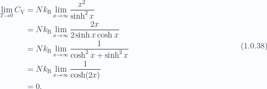
Classical limits
In the high temperature limit  , we have


so

or

matching the classical result of eq. 1.0.23. Similarly from the quantum specific heat result of eq. 1.0.31, we have

This matches our classical result from eq. 1.0.24. We expect this equivalence at high temperatures since our quantum harmonic partition function eq. 1.0.26 is approximately

This differs from the classical partition function only by this factor of  . While this alters the free energy by
  , it doesn’t change the mean energy since
  . At high temperatures the mean energy are large enough that the quantum nature of the system has no significant effect.
Low temperature limits
For the classical case the heat capacity was constant ( ), all the way down to zero. For the quantum case the heat capacity drops to zero for low temperatures. We can see that via L’hopitals rule. With
  the low temperature limit is
We also see this in the plot of fig. 1.2.

Fig 1.2: Specific heat for N quantum oscillators
Question: Quantum electric dipole (2013 problem set 5, p3)
A quantum electric dipole at a fixed space point has its energy determined by two parts – a part which comes from its angular motion and a part coming from its interaction with an applied electric field  . This leads to a quantum Hamiltonian

where  is the moment of inertia, and we have assumed an electric field
  . This Hamiltonian has eigenstates described by spherical harmonics
  , with
  taking on
  possible integral values,
  . The corresponding eigenvalues are

(Recall that  is the total angular momentum eigenvalue, while is the eigenvalue corresponding to
  .)
.)
Part a
Schematically sketch these eigenvalues as a function of for  .
.
Part b
Find the quantum partition function, assuming only  and
and  contribute to the sum.
Part c
Using this partition function, find the average dipole moment  as a function of the electric field and temperature for small electric fields, commenting on its behavior at very high temperature and very low temperature.
Part d
Estimate the temperature above which discarding higher angular momentum states, with  , is not a good approximation.
Answer
Sketch the energy eigenvalues
Let’s summarize the values of the energy eigenvalues  for
for  before attempting to plot them.
For , the azimuthal quantum number can only take the value  , so we have

For we have

so we have


For we have

so we have


These are sketched as a function of in fig. 1.3.

Fig 1.3: Energy eigenvalues for l = 0,1, 2
Partition function
Our partition function, in general, is
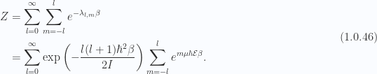
Dropping all but  terms this is

or

Average dipole moment
For the average dipole moment, averaging over both the states and the partitions, we have
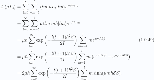
For the cap of we have

or

This is plotted in fig. 1.4.

Fig 1.4: Dipole moment
For high temperatures  or
or  , expanding the hyperbolic sine and cosines to first and second order respectively and the exponential to first order we have

Our dipole moment tends to zero approximately inversely proportional to temperature. These last two respective approximations are plotted along with the all temperature range result in fig. 1.5.

Fig 1.5: High temperature approximations to dipole moments
For low temperatures  , where
  we have

Provided the electric field is small enough (which means here that  ) this will look something like fig. 1.6.

Fig 1.6: Low temperature dipole moment behavior
Approximation validation
In order to validate the approximation, let’s first put the partition function and the numerator of the dipole moment into a tidier closed form, evaluating the sums over the radial indices . First let’s sum the exponentials for the partition function, making an 

With a substitution of  , we have
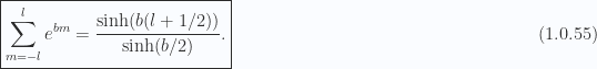
Now we can sum the azimuthal exponentials for the dipole moment. This sum is of the form

With  , and
, and  , we have

we have

With a little help from Mathematica to simplify that result we have

We can now express the average dipole moment with only sums over radial indices

So our average dipole moment is

The hyperbolic sine in the denominator from the partition function and the difference of hyperbolic sines in the numerator both grow fast. This is illustrated in fig. 1.7.

Fig 1.7: Hyperbolic sine plots for dipole moment
Let’s look at the order of these hyperbolic sines for large arguments. For the numerator we have a difference of the form

For the hyperbolic sine from the partition function we have for large 

While these hyperbolic sines increase without bound as increases, we have a negative quadratic dependence on in the  contribution to these sums, provided that is small enough we can neglect the linear growth of the hyperbolic sines. We wish for that factor to be large enough that it dominates for all . That is

or

Observe that the RHS of this inequality, for  satisfies

So, for small electric fields, our approximation should be valid provided our temperature is constrained by


 . Is the state
 is given by Eq. (9.60),
  is a constant, and time
  , an energy eigenstate of the system? What is probability per unit length for measuring the particle at position
  at
at  ? Explain the physical meaning of the above results.
 ,
,  , and
, and  . With this variable substitution Schr\”{o}dinger’s equation for this harmonic oscillator potential takes the form
 into this to get
 , this isn’t a normalizable wavefunction, and has no physical relevance, unless we set
  .
. latex x < a$} \\ \frac{1}{{2}} K x^2 & \quad \mbox{if $latex a < x b$} \\ \end{array}\right.\end{aligned} \hspace{\stretch{1}}(2.3)$
 , for constant
  . For such a potential, within the harmonic well, a general solution of the form
 values in that situation. For the wave function to be a physically relevant, we require it to be (absolute) square integrable, and must also integrate to unity over the entire interval.
 (that probability is zero in a continuous space), but we can answer the question for the probability that a particle is found in an interval surrounding a specific point at this time. By calculating the average of the probability to find the particle in an interval, and dividing by that interval’s length, we arrive at plausible definition of probability per unit length for an interval surrounding
 latex x = x_0$} =\lim_{\epsilon \rightarrow 0} \frac{1}{{\epsilon}} \int_{x_0 – \epsilon/2}^{x_0 + \epsilon/2} {\left\lvert{ \Psi(x, t_0) }\right\rvert}^2 dx = {\left\lvert{\Psi(x_0, t_0)}\right\rvert}^2\end{aligned} \hspace{\stretch{1}}(2.5)$
 wavefunction 2.1. Since normalization requires
  , that probability density is simply zero (or undefined, depending on one’s point of view).
 coefficients yield unit probability
 , we have
 we have just
 . For even
  may equal
  (this is true at least up to n=4). If that’s the case, we have for non-mixed states, with even numbered energy quantum numbers, at
  .
.