[Click here for a PDF of this post with nicer formatting (especially if my latex to wordpress script has left FORMULA DOES NOT PARSE errors.)]
Disclaimer
Peeter’s lecture notes from class. May not be entirely coherent.
Fermions summary
We’ve considered a momentum sphere as in fig. 1.1, and performed various appromations of the occupation sums fig. 1.2.

Fig 1.1: Summation over momentum sphere

Fig 1.2: Fermion occupation


The physics of Fermi gases has an extremely wide range of applicability. Illustrating some of this range, here are some examples of Fermi temperatures (from  )
)
- Electrons in copper:

- Neutrons in neutron star:

- Ultracold atomic gases:

Bosons
We’d like to work with a fixed number of particles, but the calculations are hard, so we move to the grand canonical ensemble

Again, we’ll consider free particles with energy as in fig. 1.3, or


Fig 1.3: Free particle energy momentum distribution
Again introducing fugacity  , we have

We’ll consider systems for which

Observe that at large energies we have

For small energies

Observe that we require  (or
(or  ) so that the number distribution is strictly positive for all energies. This tells us that the fugacity is a function of temperature, but there will be a point at which it must saturate. This is illustrated in fig. 1.4.

Fig 1.4: Density times cubed thermal de Broglie wavelength
Let’s calculate this density (assumed fixed for all temperatures)
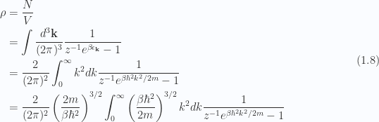
With the substitution

we find
This implicitly defines a relationship for the fugacity as a function of temperature  .
.
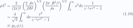
It can be shown that

As  we end up with a zeta function, for which we can look up the value

where the Riemann zeta function is defined as


At high temperatures we have

(as  does down,
  goes up)
Looking at 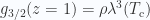 leads to
How do I satisfy number conservation?
We have a problem here since as  the
the  term in
  above drops to zero, yet
  cannot keep increasing without bounds to compensate and keep the density fixed. The way to deal with this was worked out by
- Bose (1924) for photons (examining statistics for symmetric wave functions).
- Einstein (1925) for conserved particles.
To deal with this issue, we (somewhat arbitrarily, because we need to) introduce a non-zero density for  . This is an adjustment of the approximation so that we have

as in fig. 1.5, so that

Fig 1.5: Momentum sphere with origin omitted

Given this, we have

We can illustrate this as in fig. 1.6.

Fig 1.6: Boson occupation vs momentum

At  we have
  , whereas at
  we must introduce a non-zero density if we want to be able to keep a constant density constraint.
 . Unlike photons or phonons, these particles are {\bf conserved}, and hence we must determine the chemical potential
  which fixes their density. Working in three dimensions, show whether or not these particles will exhibit Bose condensation, and find
  if it is nonzero.


 , a fixed number. The key feature of Bose condensation remains. There is a finite limit to the number of particles that can be in the energetic state at a given temperature and volume. Any remaining particles are forced into the ground state.

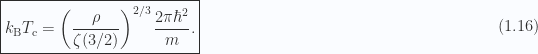
 is the Bose condensation temperature
 ,
,  , we have for the ground state average number density


