[Click here for a PDF of this post with nicer formatting]
Motivation.
Chapter V notes for [1].
Notes
Problems
Problem 1.
Statement.
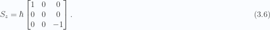
Obtain  for spin 1 in the representation in which
  and
and  are diagonal.
Solution.
For spin 1, we have

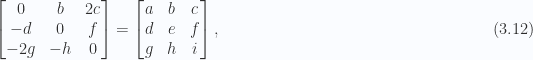
and are interested in the states  . If, like angular momentum, we assume that we have for

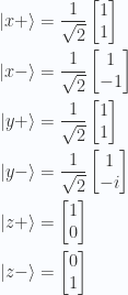
and introduce a column matrix representations for the kets as follows

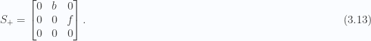
then we have, by inspection
Note that, like the Pauli matrices, and unlike angular momentum, the spin states 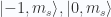 have not been considered. Do those have any physical interpretation?
That question aside, we can proceed as in the text, utilizing the ladder operator commutators

to determine the values of  and
and  indirectly. We find
![\begin{aligned}\left[{S_{+}},{S_{-}}\right] &= 2 \hbar S_z \\ \left[{S_{+}},{S_{z}}\right] &= -\hbar S_{+} \\ \left[{S_{-}},{S_{z}}\right] &= \hbar S_{-}.\end{aligned} \hspace{\stretch{1}}(3.8)](https://s0.wp.com/latex.php?latex=%5Cbegin%7Baligned%7D%5Cleft%5B%7BS_%7B%2B%7D%7D%2C%7BS_%7B-%7D%7D%5Cright%5D+%26%3D+2+%5Chbar+S_z+%5C%5C+%5Cleft%5B%7BS_%7B%2B%7D%7D%2C%7BS_%7Bz%7D%7D%5Cright%5D+%26%3D+-%5Chbar+S_%7B%2B%7D+%5C%5C+%5Cleft%5B%7BS_%7B-%7D%7D%2C%7BS_%7Bz%7D%7D%5Cright%5D+%26%3D+%5Chbar+S_%7B-%7D.%5Cend%7Baligned%7D+%5Chspace%7B%5Cstretch%7B1%7D%7D%283.8%29&bg=fafcff&fg=2a2a2a&s=0&c=20201002)
Let
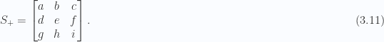
Looking for equality between ![\left[{S_{z}},{S_{+}}\right]/\hbar = S_{+}](https://s0.wp.com/latex.php?latex=%5Cleft%5B%7BS_%7Bz%7D%7D%2C%7BS_%7B%2B%7D%7D%5Cright%5D%2F%5Chbar+%3D+S_%7B%2B%7D&bg=fafcff&fg=2a2a2a&s=0&c=20201002) , we find
, we find
so we must have
Furthermore, from ![\left[{S_{+}},{S_{-}}\right] = 2 \hbar S_z](https://s0.wp.com/latex.php?latex=%5Cleft%5B%7BS_%7B%2B%7D%7D%2C%7BS_%7B-%7D%7D%5Cright%5D+%3D+2+%5Chbar+S_z&bg=fafcff&fg=2a2a2a&s=0&c=20201002) , we find
, we find

We must have 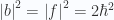 . We could probably pick any
 , and
, and  , but assuming we have no reason for a non-zero phase we try
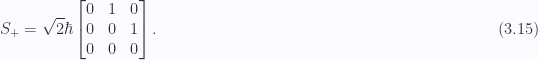
Putting all the pieces back together, with 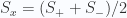 , and
, and  , we finally have

A quick calculation verifies that we have 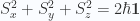 , as expected.
Problem 2.
Statement.
Obtain eigensolution for operator  . Call the eigenstates
  and
and  , and determine the probabilities that they will correspond to
  .
.
Solution.
The first part is straight forward, and we have
Taking  we get

with eigenvectors proportional to

The normalization constant is  . Now we can call these , and but what does the last part of the question mean? What’s meant by ?
Asking the prof about this, he says:
“I think it means that the result of a measurement of the x component of spin is  . This corresponds to the eigenvalue of
  being . The spin operator has eigenvalue
  ”.
”.
Aside: Question to consider later. Is is significant that 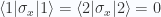 ?
?
So, how do we translate this into a mathematical statement?
First let’s recall a couple of details. Recall that the x spin operator has the matrix representation

This has eigenvalues  , with eigenstates
  . At the point when the x component spin is observed to be , the state of the system was then

Let’s look at the ways that this state can be formed as linear combinations of our states , and . That is

or

Letting  , this is

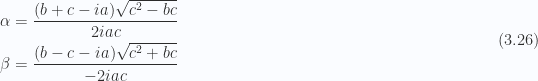
We can solve the  and
and  with Cramer’s rule, yielding
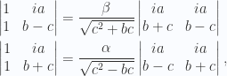
or
It is  and
and  that are probabilities, and after a bit of algebra we find that those are

so if the x spin of the system is measured as , we have a $50\
Is that what the question was asking? I think that I’ve actually got it backwards. I think that the question was asking for the probability of finding state  (measuring a spin 1 value for ) given the state or .
So, suppose that we have

or (considering both cases simultaneously),

or

Unsurprisingly, this mirrors the previous scenario and we find that we have a probability  of measuring a spin 1 value for when the state of the operator
  has been measured as
  (ie: in the states , or respectively).
No measurement of the operator 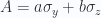 gives a biased prediction of the state of the state . Loosely, this seems to justify calling these operators orthogonal. This is consistent with the geometrical antisymmetric nature of the spin components where we have
  , just like two orthogonal vectors under the Clifford product.
Problem 3.
Statement.
Obtain the expectation values of for the case of a spin  particle with the spin pointed in the direction of a vector with azimuthal angle and polar angle .
Solution.
Let’s work with  instead of
  to eliminate the
  factors. Before considering the expectation values in the arbitrary spin orientation, let’s consider just the expectation values for . Introducing a matrix representation (assumed normalized) for a reference state

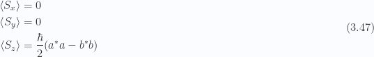
we find
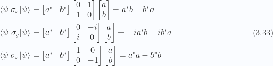
Each of these expectation values are real as expected due to the Hermitian nature of . We also find that

So a vector formed with the expectation values as components is a unit vector. This doesn’t seem too unexpected from the section on the projection operators in the text where it was stated that  , where
  was a unit vector, and this seems similar. Let’s now consider the arbitrarily oriented spin vector
  , and look at its expectation value.
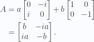
With  as the the rotated image of
  by an azimuthal angle , and polar angle , we have

that is

The  projections of this operator

are just the Pauli matrices scaled by the components of
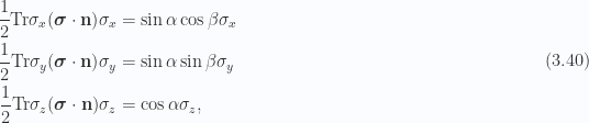
so our expectation values are by inspection
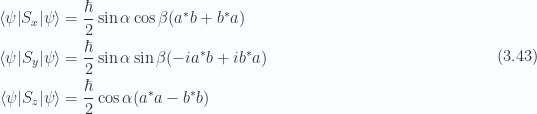
Is this correct? While  is a unit norm operator, we find that the expectation values of the coordinates of cannot be viewed as the coordinates of a unit vector. Let’s consider a specific case, with
  , where the spin is oriented in the
  plane. That gives us

so the expectation values of are
Given this is seems reasonable that from 3.43 we find

(since we don’t have any reason to believe that in general  is true).
The most general statement we can make about these expectation values (an average observed value for the measurement of the operator) is that

with equality for specific states and orientations only.
Problem 4.
Statement.
Take the azimuthal angle,  , so that the spin is in the
x-z plane at an angle with respect to the z-axis, and the unit vector is 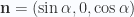 . Write

for this case. Show that the probability that it is in the spin-up state in the direction  with respect to the z-axis is

Also obtain the expectation value of with respect to the state  .
.
Solution.
For this orientation we have

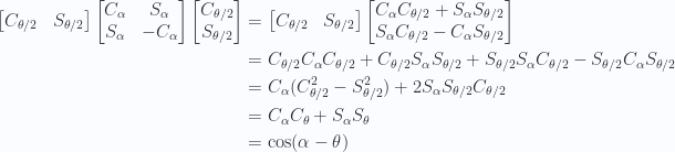
Confirmation that our eigenvalues are is simple, and our eigenstates for the eigenvalue is found to be

This last has unit norm, so we can write

If the state has been measured to be

then the probability of a second measurement obtaining is

Expanding just the inner product first we have

So our probability of measuring spin up state given the state was known to have been in spin up state  is
is

Finally, the expectation value for with respect to is
Sanity checking this we observe that we have as desired for the  case.
case.
Problem 5.
Statement.
Consider an arbitrary density matrix,  , for a spin system. Express each matrix element in terms of the ensemble averages
 ![[S_i]](https://s0.wp.com/latex.php?latex=%5BS_i%5D&bg=fafcff&fg=2a2a2a&s=0&c=20201002) where
where  .
.
Solution.
Let’s omit the spin direction temporarily and write for the density matrix
For the ensemble average (no sum over repeated indexes) we have
![\begin{aligned}[S] = \left\langle{{S}}\right\rangle_{av} &= w_{+} {\langle {+} \rvert} S {\lvert {+} \rangle} +w_{-} {\langle {-} \rvert} S {\lvert {-} \rangle} \\ &= \frac{\hbar}{2}( w_{+} -w_{-} ) \\ &= \frac{\hbar}{2}( w_{+} -(1 - w_{+}) ) \\ &= \hbar w_{+} - \frac{1}{{2}}\end{aligned}](https://s0.wp.com/latex.php?latex=%5Cbegin%7Baligned%7D%5BS%5D+%3D+%5Cleft%5Clangle%7B%7BS%7D%7D%5Cright%5Crangle_%7Bav%7D+%26%3D+w_%7B%2B%7D+%7B%5Clangle+%7B%2B%7D+%5Crvert%7D+S+%7B%5Clvert+%7B%2B%7D+%5Crangle%7D+%2Bw_%7B-%7D+%7B%5Clangle+%7B-%7D+%5Crvert%7D+S+%7B%5Clvert+%7B-%7D+%5Crangle%7D+%5C%5C+%26%3D+%5Cfrac%7B%5Chbar%7D%7B2%7D%28+w_%7B%2B%7D+-w_%7B-%7D+%29+%5C%5C+%26%3D+%5Cfrac%7B%5Chbar%7D%7B2%7D%28+w_%7B%2B%7D+-%281+-+w_%7B%2B%7D%29+%29+%5C%5C+%26%3D+%5Chbar+w_%7B%2B%7D+-+%5Cfrac%7B1%7D%7B%7B2%7D%7D%5Cend%7Baligned%7D+&bg=fafcff&fg=2a2a2a&s=0&c=20201002)
This gives us
![\begin{aligned}w_{+} = \frac{1}{{\hbar}} [S] + \frac{1}{{2}}\end{aligned}](https://s0.wp.com/latex.php?latex=%5Cbegin%7Baligned%7Dw_%7B%2B%7D+%3D+%5Cfrac%7B1%7D%7B%7B%5Chbar%7D%7D+%5BS%5D+%2B+%5Cfrac%7B1%7D%7B%7B2%7D%7D%5Cend%7Baligned%7D+&bg=fafcff&fg=2a2a2a&s=0&c=20201002)
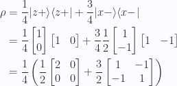
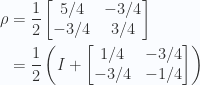
and our density matrix becomes
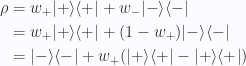
![\begin{aligned}\rho &=\frac{1}{{2}} ( {\lvert {+} \rangle}{\langle {+} \rvert} +{\lvert {-} \rangle}{\langle {-} \rvert} )+\frac{1}{{\hbar}} [S] ({\lvert {+} \rangle}{\langle {+} \rvert} -{\lvert {+} \rangle}{\langle {+} \rvert}) \\ &=\frac{1}{{2}} I+\frac{1}{{\hbar}} [S] ({\lvert {+} \rangle}{\langle {+} \rvert} -{\lvert {+} \rangle}{\langle {+} \rvert}) \\ \end{aligned}](https://s0.wp.com/latex.php?latex=%5Cbegin%7Baligned%7D%5Crho+%26%3D%5Cfrac%7B1%7D%7B%7B2%7D%7D+%28+%7B%5Clvert+%7B%2B%7D+%5Crangle%7D%7B%5Clangle+%7B%2B%7D+%5Crvert%7D+%2B%7B%5Clvert+%7B-%7D+%5Crangle%7D%7B%5Clangle+%7B-%7D+%5Crvert%7D+%29%2B%5Cfrac%7B1%7D%7B%7B%5Chbar%7D%7D+%5BS%5D+%28%7B%5Clvert+%7B%2B%7D+%5Crangle%7D%7B%5Clangle+%7B%2B%7D+%5Crvert%7D+-%7B%5Clvert+%7B%2B%7D+%5Crangle%7D%7B%5Clangle+%7B%2B%7D+%5Crvert%7D%29+%5C%5C+%26%3D%5Cfrac%7B1%7D%7B%7B2%7D%7D+I%2B%5Cfrac%7B1%7D%7B%7B%5Chbar%7D%7D+%5BS%5D+%28%7B%5Clvert+%7B%2B%7D+%5Crangle%7D%7B%5Clangle+%7B%2B%7D+%5Crvert%7D+-%7B%5Clvert+%7B%2B%7D+%5Crangle%7D%7B%5Clangle+%7B%2B%7D+%5Crvert%7D%29+%5C%5C+%5Cend%7Baligned%7D+&bg=fafcff&fg=2a2a2a&s=0&c=20201002)
Utilizing
We can easily find

So we can write the density matrix in terms of any of the ensemble averages as
![\begin{aligned}\rho =\frac{1}{{2}} I+\frac{1}{{\hbar}} [S_i] \sigma_i=\frac{1}{{2}} (I + [\sigma_i] \sigma_i )\end{aligned}](https://s0.wp.com/latex.php?latex=%5Cbegin%7Baligned%7D%5Crho+%3D%5Cfrac%7B1%7D%7B%7B2%7D%7D+I%2B%5Cfrac%7B1%7D%7B%7B%5Chbar%7D%7D+%5BS_i%5D+%5Csigma_i%3D%5Cfrac%7B1%7D%7B%7B2%7D%7D+%28I+%2B+%5B%5Csigma_i%5D+%5Csigma_i+%29%5Cend%7Baligned%7D+&bg=fafcff&fg=2a2a2a&s=0&c=20201002)
Alternatively, defining ![\mathbf{P}_i = [\sigma_i] \mathbf{e}_i](https://s0.wp.com/latex.php?latex=%5Cmathbf%7BP%7D_i+%3D+%5B%5Csigma_i%5D+%5Cmathbf%7Be%7D_i&bg=fafcff&fg=2a2a2a&s=0&c=20201002) , for any of the directions
, for any of the directions  we can write

In equation (5.109) we had a similar result in terms of the polarization vector  , and the individual weights
  , and
, and  , but we see here that this
  factor can be written exclusively in terms of the ensemble average. Actually, this is also a result in the text, down in (5.113), but we see it here in a more concrete form having picked specific spin directions.
Problem 6.
Statement.
If a Hamiltonian is given by where  , determine the time evolution operator as a 2 x 2 matrix. If a state at
  is given by

then obtain  .
.
Solution.
Before diving into the meat of the problem, observe that a tidy factorization of the Hamiltonian is possible as a composition of rotations. That is
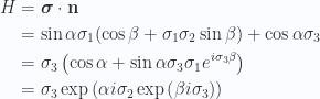
So we have for the time evolution operator

Does this really help? I guess not, but it is nice and tidy.
Returning to the specifics of the problem, we note that squaring the Hamiltonian produces the identity matrix

This allows us to exponentiate  by inspection utilizing

Writing  , and
, and  , we have

and thus

Note that as a sanity check we can calculate that  as expected.
Now for  , we have

It doesn’t seem terribly illuminating to multiply this all out, but we can factor the results slightly to tidy it up. That gives us

Problem 7.
Statement.
Consider a system of spin particles in a mixed ensemble containing a mixture of 25\
Solution.
We have
Giving us

Note that we can also factor the identity out of this for
which is just:

Recall that the ensemble average is related to the trace of the density and operator product

But this, by definition of the ensemble average, is just

We can use this to compute the ensemble averages of the Pauli matrices

We can also find without the explicit matrix multiplication from 3.70

(where to do so we observe that  for
for  and
and  , and
, and  .)
.)
We see that the traces of the density operator and Pauli matrix products act very much like dot products extracting out the ensemble averages, which end up very much like the magnitudes of the projections in each of the directions.
Problem 8.
Statement.
Show that the quantity  , when simplified, has a term proportional to
  .
.
Solution.
Consider the operation

With  , we have

which gives us the commutator
![\begin{aligned}\left[{ \boldsymbol{\sigma} \cdot \mathbf{p}},{V(r)}\right]&=- \frac{i \hbar}{r} \frac{\partial {V(r)}}{\partial {r}} (\boldsymbol{\sigma} \cdot \mathbf{x}) \end{aligned} \hspace{\stretch{1}}(3.72)](https://s0.wp.com/latex.php?latex=%5Cbegin%7Baligned%7D%5Cleft%5B%7B+%5Cboldsymbol%7B%5Csigma%7D+%5Ccdot+%5Cmathbf%7Bp%7D%7D%2C%7BV%28r%29%7D%5Cright%5D%26%3D-+%5Cfrac%7Bi+%5Chbar%7D%7Br%7D+%5Cfrac%7B%5Cpartial+%7BV%28r%29%7D%7D%7B%5Cpartial+%7Br%7D%7D+%28%5Cboldsymbol%7B%5Csigma%7D+%5Ccdot+%5Cmathbf%7Bx%7D%29+%5Cend%7Baligned%7D+%5Chspace%7B%5Cstretch%7B1%7D%7D%283.72%29&bg=fafcff&fg=2a2a2a&s=0&c=20201002)
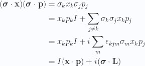
Insertion into the operator in question we have

With decomposition of the  into symmetric and antisymmetric components, we should have in the second term our
![\begin{aligned}(\boldsymbol{\sigma} \cdot \mathbf{x}) (\boldsymbol{\sigma} \cdot \mathbf{p} )=\frac{1}{{2}} \left\{{\boldsymbol{\sigma} \cdot \mathbf{x}},{\boldsymbol{\sigma} \cdot \mathbf{p}}\right\}+\frac{1}{{2}} \left[{\boldsymbol{\sigma} \cdot \mathbf{x}},{\boldsymbol{\sigma} \cdot \mathbf{p}}\right]\end{aligned} \hspace{\stretch{1}}(3.74)](https://s0.wp.com/latex.php?latex=%5Cbegin%7Baligned%7D%28%5Cboldsymbol%7B%5Csigma%7D+%5Ccdot+%5Cmathbf%7Bx%7D%29+%28%5Cboldsymbol%7B%5Csigma%7D+%5Ccdot+%5Cmathbf%7Bp%7D+%29%3D%5Cfrac%7B1%7D%7B%7B2%7D%7D+%5Cleft%5C%7B%7B%5Cboldsymbol%7B%5Csigma%7D+%5Ccdot+%5Cmathbf%7Bx%7D%7D%2C%7B%5Cboldsymbol%7B%5Csigma%7D+%5Ccdot+%5Cmathbf%7Bp%7D%7D%5Cright%5C%7D%2B%5Cfrac%7B1%7D%7B%7B2%7D%7D+%5Cleft%5B%7B%5Cboldsymbol%7B%5Csigma%7D+%5Ccdot+%5Cmathbf%7Bx%7D%7D%2C%7B%5Cboldsymbol%7B%5Csigma%7D+%5Ccdot+%5Cmathbf%7Bp%7D%7D%5Cright%5D%5Cend%7Baligned%7D+%5Chspace%7B%5Cstretch%7B1%7D%7D%283.74%29&bg=fafcff&fg=2a2a2a&s=0&c=20201002)
where we expect ![\boldsymbol{\sigma} \cdot \mathbf{L} \propto \left[{\boldsymbol{\sigma} \cdot \mathbf{x}},{\boldsymbol{\sigma} \cdot \mathbf{p}}\right]](https://s0.wp.com/latex.php?latex=%5Cboldsymbol%7B%5Csigma%7D+%5Ccdot+%5Cmathbf%7BL%7D+%5Cpropto+%5Cleft%5B%7B%5Cboldsymbol%7B%5Csigma%7D+%5Ccdot+%5Cmathbf%7Bx%7D%7D%2C%7B%5Cboldsymbol%7B%5Csigma%7D+%5Ccdot+%5Cmathbf%7Bp%7D%7D%5Cright%5D&bg=fafcff&fg=2a2a2a&s=0&c=20201002) . Alternately in components
. Alternately in components
Problem 9.
Statement.
Solution.
TODO.
References
[1] BR Desai. Quantum mechanics with basic field theory. Cambridge University Press, 2009.


 , all available phase space will be covered. Not all systems are necessarily ergodic, but the hope is that all sufficiently complicated systems will be so.
 , we see that our continuity equation 1.2.1 results in 1.2.2.


 is the allowed “volume” of phase space, the number of states that the system can take that is consistent with conservation of energy.
 gas atoms at phase space points

 .
.
 defined implicitly by


 , the dimension of momentum part of the phase space is 3. In general the dimension of the space is
  . Here


 .
. , where
  is Plank’s constant.
 , the question of how many boxes there are, we calculate the total volume, and then divide by the volume of each box. This sort of handwaving wouldn’t be required if we did a proper quantum mechanical treatment.

