Peeter Joot's (OLD) Blog.

Math, physics, perl, and programming obscurity.

Verifying the Helmholtz Green’s function.

Posted by peeterjoot on December 9, 2011

[Click here for a PDF of this post with nicer formatting and figures if the post had any (especially if my latex to wordpress script has left FORMULA DOES NOT PARSE errors.)]

Motivation.

In class this week, looking at an instance of the Helmholtz equation

\begin{aligned}\left( \boldsymbol{\nabla}^2 + \mathbf{k}^2\right) \psi_\mathbf{k}(\mathbf{r}) = s(\mathbf{r}).\end{aligned} \hspace{\stretch{1}}(1.1)

We were told that the Green’s function

\begin{aligned}\left( \boldsymbol{\nabla}^2 + \mathbf{k}^2\right) G^0(\mathbf{r}, \mathbf{r}') = \delta(\mathbf{r}- \mathbf{r}')\end{aligned} \hspace{\stretch{1}}(1.2)

that can be used to solve for a particular solution this differential equation via convolution

\begin{aligned}\psi_\mathbf{k}(\mathbf{r}) = \int G^0(\mathbf{r}, \mathbf{r}') s(\mathbf{r}') d^3 \mathbf{r}',\end{aligned} \hspace{\stretch{1}}(1.3)

had the value

\begin{aligned}G^0(\mathbf{r}, \mathbf{r}') = - \frac{1}{{4 \pi}} \frac{e^{i k {\left\lvert{\mathbf{r} - \mathbf{r}'}\right\rvert}} }{{\left\lvert{\mathbf{r} - \mathbf{r}'}\right\rvert}}.\end{aligned} \hspace{\stretch{1}}(1.4)

Let’s try to verify this.

Guts

Application of the Helmholtz differential operator \boldsymbol{\nabla}^2 + \mathbf{k}^2 on the presumed solution gives

\begin{aligned}(\boldsymbol{\nabla}^2 + \mathbf{k}^2) \psi_\mathbf{k}(\mathbf{r}) = - \frac{1}{{4 \pi}} \int (\boldsymbol{\nabla}^2 + \mathbf{k}^2) \frac{e^{i k {\left\lvert{\mathbf{r} - \mathbf{r}'}\right\rvert}} }{{\left\lvert{\mathbf{r} - \mathbf{r}'}\right\rvert}}s(\mathbf{r}') d^3 \mathbf{r}'.\end{aligned} \hspace{\stretch{1}}(2.5)

When \mathbf{r} \ne \mathbf{r}'.

To proceed we’ll need to evaluate

\begin{aligned}\boldsymbol{\nabla}^2 \frac{e^{i k {\left\lvert{\mathbf{r} - \mathbf{r}'}\right\rvert}} }{{\left\lvert{\mathbf{r} - \mathbf{r}'}\right\rvert}}.\end{aligned} \hspace{\stretch{1}}(2.6)

Writing \mu = {\left\lvert{\mathbf{r} - \mathbf{r}'}\right\rvert} we start with the computation of

\begin{aligned}\frac{\partial {}}{\partial {x}} \frac{e^{i k \mu} }{\mu}&=\frac{\partial {\mu}}{\partial {x}} \left( \frac{i k}{\mu} - \frac{1}{{\mu^2}} \right) e^{i k \mu} \\ &=\frac{\partial {\mu}}{\partial {x}} \left( i k - \frac{1}{{\mu}} \right) \frac{e^{i k \mu}}{\mu}\end{aligned}

We see that we’ll have

\begin{aligned}\boldsymbol{\nabla} \frac{e^{i k \mu} }{\mu} = \left( i k - \frac{1}{{\mu}} \right) \frac{e^{i k \mu}}{\mu} \boldsymbol{\nabla} \mu.\end{aligned} \hspace{\stretch{1}}(2.7)

Taking second derivatives with respect to x we find

\begin{aligned}\frac{\partial^2 {{}}}{\partial {{x}}^2} \frac{e^{i k \mu} }{\mu}&=\frac{\partial^2 {{\mu}}}{\partial {{x}}^2} \left( i k - \frac{1}{{\mu}} \right) \frac{e^{i k \mu}}{\mu}+\frac{\partial {\mu}}{\partial {x}} \frac{\partial {\mu}}{\partial {x}} \frac{1}{{\mu^2}} \frac{e^{i k \mu}}{\mu}+\left( \frac{\partial {\mu}}{\partial {x}} \right)^2 \left( i k - \frac{1}{{\mu}} \right)^2 \frac{e^{i k \mu}}{\mu} \\ &=\frac{\partial^2 {{\mu}}}{\partial {{x}}^2} \left( i k - \frac{1}{{\mu}} \right) \frac{e^{i k \mu}}{\mu}+\left( \frac{\partial {\mu}}{\partial {x}} \right)^2 \left( -k^2 - \frac{ 2 i k }{\mu} + \frac{2}{\mu^2} \right)\frac{e^{i k \mu}}{\mu}.\end{aligned}

Our Laplacian is then

\begin{aligned}\boldsymbol{\nabla}^2\frac{e^{i k \mu} }{\mu} =\left( i k - \frac{1}{{\mu}} \right) \frac{e^{i k \mu}}{\mu} \boldsymbol{\nabla}^2 \mu+\left( -k^2 - \frac{ 2 i k }{\mu} + \frac{2}{\mu^2} \right)\frac{e^{i k \mu}}{\mu} (\boldsymbol{\nabla} \mu)^2.\end{aligned} \hspace{\stretch{1}}(2.8)

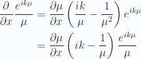
Now lets calculate the derivatives of \mu. Working on x again, we have

\begin{aligned}\frac{\partial {}}{\partial {x}} \mu&=\frac{\partial {}}{\partial {x}} \sqrt{ (x - x')^2 +(y - y')^2 +(z - z')^2 } \\ &=\frac{1}{{2}} 2 (x - x')\frac{1}{{\sqrt{ (x - x')^2 +(y - y')^2 +(z - z')^2 }}} \\ &=\frac{x - x'}{\mu}.\end{aligned}

So we have

\begin{aligned}\boldsymbol{\nabla} \mu &= \frac{\mathbf{r} - \mathbf{r}'}{\mu} \\ (\boldsymbol{\nabla} \mu)^2 &= 1 \end{aligned} \hspace{\stretch{1}}(2.9)

Taking second derivatives with respect to x we find

\begin{aligned}\frac{\partial^2 {{}}}{\partial {{x}}^2} \mu&= \frac{\partial {}}{\partial {x}}\frac{x - x'}{\mu} \\ &= \frac{1}{\mu} - (x - x') \frac{\partial {\mu}}{\partial {x}} \frac{1}{{\mu^2}}\\ &=\frac{1}{\mu} - (x - x') \frac{x - x'}{\mu} \frac{1}{{\mu^2}}\\ &=\frac{1}{\mu} - (x - x')^2 \frac{1}{{\mu^3}}.\end{aligned}

So we find

\begin{aligned}\boldsymbol{\nabla}^2 \mu = \frac{3}{\mu} - \frac{1}{{\mu}},\end{aligned} \hspace{\stretch{1}}(2.11)

or

\begin{aligned}\boldsymbol{\nabla}^2 \mu = \frac{2}{\mu}.\end{aligned} \hspace{\stretch{1}}(2.12)

Inserting this and (\boldsymbol{\nabla} \mu)^2 into 2.8 we find

\begin{aligned}\begin{aligned}\boldsymbol{\nabla}^2\frac{e^{i k \mu} }{\mu} &=\left( i k - \frac{1}{{\mu}} \right) \frac{e^{i k \mu}}{\mu} \frac{2}{\mu}+\left( -k^2 - \frac{ 2 i k }{\mu} + \frac{2}{\mu^2} \right)\frac{e^{i k \mu}}{\mu}&=-k^2 \frac{e^{i k \mu}}{\mu}\end{aligned}\end{aligned} \hspace{\stretch{1}}(2.13)

This shows us that provided \mathbf{r} \ne \mathbf{r}' we have

\begin{aligned}(\boldsymbol{\nabla}^2 + \mathbf{k}^2) G^0(\mathbf{r}, \mathbf{r}') = 0.\end{aligned} \hspace{\stretch{1}}(2.14)

In the neighborhood of {\left\lvert{\mathbf{r} - \mathbf{r}'}\right\rvert} < \epsilon.

Having shown that we end up with zero everywhere that \mathbf{r} \ne \mathbf{r}' we are left to consider a neighborhood of the volume surrounding the point \mathbf{r} in our integral. Following the Coulomb treatment in section 2.2 of [1] we use a spherical volume element centered around \mathbf{r} of radius \epsilon, and then convert a divergence to a surface area to evaluate the integral away from the problematic point

\begin{aligned}-\frac{1}{{4\pi}} \int_{\text{all space}} (\boldsymbol{\nabla}^2 + \mathbf{k}^2) \frac{e^{i k {\left\lvert{\mathbf{r} - \mathbf{r}'}\right\rvert}}}{{\left\lvert{\mathbf{r} - \mathbf{r}'}\right\rvert}} s(\mathbf{r}') d^3 \mathbf{r}'=-\frac{1}{{4\pi}} \int_{{\left\lvert{\mathbf{r} - \mathbf{r}'}\right\rvert} < \epsilon} (\boldsymbol{\nabla}^2 + \mathbf{k}^2) \frac{e^{i k {\left\lvert{\mathbf{r} - \mathbf{r}'}\right\rvert}}}{{\left\lvert{\mathbf{r} - \mathbf{r}'}\right\rvert}} s(\mathbf{r}') d^3 \mathbf{r}'\end{aligned} \hspace{\stretch{1}}(2.15)

We make the change of variables \mathbf{r}' = \mathbf{r} + \mathbf{a}. We add an explicit \mathbf{r} suffix to our Laplacian at the same time to remind us that it is taking derivatives with respect to the coordinates of \mathbf{r} = (x, y, z), and not the coordinates of our integration variable \mathbf{a} = (a_x, a_y, a_z). Assuming sufficient continuity and “well behavedness” of s(\mathbf{r}') we’ll be able to pull it out of the integral, giving

\begin{aligned}-\frac{1}{{4\pi}} \int_{{\left\lvert{\mathbf{r} - \mathbf{r}'}\right\rvert} < \epsilon} (\boldsymbol{\nabla}_\mathbf{r}^2 + \mathbf{k}^2) \frac{e^{i k {\left\lvert{\mathbf{r} - \mathbf{r}'}\right\rvert}}}{{\left\lvert{\mathbf{r} - \mathbf{r}'}\right\rvert}} s(\mathbf{r}') d^3 \mathbf{r}'&= -\frac{1}{4\pi} \int_{{\left\lvert{\mathbf{a}}\right\rvert} < \epsilon} (\boldsymbol{\nabla}_\mathbf{r}^2 + \mathbf{k}^2) \frac{e^{i k {\left\lvert{\mathbf{a}}\right\rvert}}}{{\left\lvert{\mathbf{a}}\right\rvert}} s(\mathbf{r} + \mathbf{a}) d^3 \mathbf{a} \\ &= -\frac{s(\mathbf{r})}{4\pi} \int_{{\left\lvert{\mathbf{a}}\right\rvert} < \epsilon} (\boldsymbol{\nabla}_\mathbf{r}^2 + \mathbf{k}^2) \frac{e^{i k {\left\lvert{\mathbf{a}}\right\rvert}}}{{\left\lvert{\mathbf{a}}\right\rvert}} d^3 \mathbf{a} \end{aligned}

Recalling the dependencies on the derivatives of {\left\lvert{\mathbf{r} - \mathbf{r}'}\right\rvert} in our previous gradient evaluations, we note that we have

\begin{aligned}\boldsymbol{\nabla}_\mathbf{r} {\left\lvert{\mathbf{r} - \mathbf{r}'}\right\rvert} &= -\boldsymbol{\nabla}_\mathbf{a} {\left\lvert{\mathbf{a}}\right\rvert} \\ (\boldsymbol{\nabla}_\mathbf{r} {\left\lvert{\mathbf{r} - \mathbf{r}'}\right\rvert})^2 &= (\boldsymbol{\nabla}_\mathbf{a} {\left\lvert{\mathbf{a}}\right\rvert})^2 \\ \boldsymbol{\nabla}_\mathbf{r}^2 {\left\lvert{\mathbf{r} - \mathbf{r}'}\right\rvert} &= \boldsymbol{\nabla}_\mathbf{a}^2 {\left\lvert{\mathbf{a}}\right\rvert},\end{aligned} \hspace{\stretch{1}}(2.16)

so with \mathbf{a} = \mathbf{r} - \mathbf{r}', we can rewrite our Laplacian as

\begin{aligned}\boldsymbol{\nabla}_\mathbf{r}^2 \frac{e^{i k {\left\lvert{\mathbf{r} - \mathbf{r}'}\right\rvert}}}{{\left\lvert{\mathbf{r} - \mathbf{r}'}\right\rvert}} = \boldsymbol{\nabla}_\mathbf{a}^2 \frac{e^{i k {\left\lvert{\mathbf{a}}\right\rvert}}}{{\left\lvert{\mathbf{a}}\right\rvert}} = \boldsymbol{\nabla}_\mathbf{a} \cdot \left(\boldsymbol{\nabla}_\mathbf{a} \frac{e^{i k {\left\lvert{\mathbf{a}}\right\rvert}}}{{\left\lvert{\mathbf{a}}\right\rvert}} \right)\end{aligned} \hspace{\stretch{1}}(2.19)

This gives us

\begin{aligned}-\frac{s(\mathbf{r})}{4\pi} \int_{{\left\lvert{\mathbf{a}}\right\rvert} < \epsilon} (\boldsymbol{\nabla}_\mathbf{a}^2 + \mathbf{k}^2) \frac{e^{i k {\left\lvert{\mathbf{a}}\right\rvert}}}{{\left\lvert{\mathbf{a}}\right\rvert}} d^3 \mathbf{a} &=-\frac{s(\mathbf{r})}{4\pi} \int_{dV} \boldsymbol{\nabla}_\mathbf{a} \cdot \left( \boldsymbol{\nabla}_\mathbf{a} \frac{e^{i k {\left\lvert{\mathbf{a}}\right\rvert}}}{{\left\lvert{\mathbf{a}}\right\rvert}} \right) d^3 \mathbf{a} -\frac{s(\mathbf{r})}{4\pi} \int_{dV}\mathbf{k}^2 \frac{e^{i k {\left\lvert{\mathbf{a}}\right\rvert}}}{{\left\lvert{\mathbf{a}}\right\rvert}} d^3 \mathbf{a}  \\ &=-\frac{s(\mathbf{r})}{4\pi} \int_{dA} \left( \boldsymbol{\nabla}_\mathbf{a} \frac{e^{i k {\left\lvert{\mathbf{a}}\right\rvert}}}{{\left\lvert{\mathbf{a}}\right\rvert}} \right) \cdot \hat{\mathbf{a}} d^2 \mathbf{a} -\frac{s(\mathbf{r})}{4\pi} \int_{dV}\mathbf{k}^2 \frac{e^{i k {\left\lvert{\mathbf{a}}\right\rvert}}}{{\left\lvert{\mathbf{a}}\right\rvert}} d^3 \mathbf{a} \end{aligned}

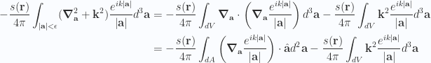
To complete these evaluations, we can now employ a spherical coordinate change of variables. Let’s do the \mathbf{k}^2 volume integral first. We have

\begin{aligned}\int_{dV}\mathbf{k}^2 \frac{e^{i k {\left\lvert{\mathbf{a}}\right\rvert}}}{{\left\lvert{\mathbf{a}}\right\rvert}} d^3 \mathbf{a} &=\int_{a = 0}^\epsilon \int_{\theta = 0}^\pi \int_{\phi=0}^{2\pi}\mathbf{k}^2 \frac{e^{i k a}}{a} a^2 da \sin\theta d\theta d\phi \\ &=4\pi k^2\int_{a = 0}^\epsilon a e^{i k a} da  \\ &=4\pi \int_{u = 0}^{k\epsilon}u e^{i u} du  \\ &=4\pi {\left.(-i u + 1) e^{i u} \right\vert}_0^{k \epsilon} \\ &=4 \pi \left( (-i k \epsilon + 1)e^{i k \epsilon} - 1 \right)\end{aligned}

To evaluate the surface integral we note that we’ll require only the radial portion of the gradient, so have

\begin{aligned}\left( \boldsymbol{\nabla}_\mathbf{a} \frac{e^{i k {\left\lvert{\mathbf{a}}\right\rvert}}}{{\left\lvert{\mathbf{a}}\right\rvert}} \right) \cdot \hat{\mathbf{a}}&=\left( \hat{\mathbf{a}} \frac{\partial {}}{\partial {a}} \frac{e^{i k a}}{a} \right) \cdot \hat{\mathbf{a}} \\ &=\frac{\partial {}}{\partial {a}} \frac{e^{i k a}}{a} \\ &=\left( i k \frac{1}{{a}} - \frac{1}{{a^2}} \right)e^{i k a} \\ &=\left( i k a - 1 \right)\frac{e^{i k a}}{a^2}\end{aligned}

Our area element is a^2 \sin\theta d\theta d\phi, so we are left with

\begin{aligned}\begin{aligned}\int_{dA} \left( \boldsymbol{\nabla}_\mathbf{a} \frac{e^{i k {\left\lvert{\mathbf{a}}\right\rvert}}}{{\left\lvert{\mathbf{a}}\right\rvert}} \right) \cdot \hat{\mathbf{a}} d^2 \mathbf{a} &={\left.{{\int_{\theta = 0}^\pi \int_{\phi=0}^{2\pi}\left( i k a - 1 \right)\frac{e^{i k a}}{a^2}a^2 \sin\theta d\theta d\phi }}\right\vert}_{{a = \epsilon}}\\ &=4 \pi\left( i k \epsilon - 1 \right) e^{i k \epsilon}\end{aligned}\end{aligned} \hspace{\stretch{1}}(2.20)

Putting everything back together we have

\begin{aligned}-\frac{1}{{4\pi}} \int_{\text{all space}} (\boldsymbol{\nabla}^2 + \mathbf{k}^2) \frac{e^{i k {\left\lvert{\mathbf{r} - \mathbf{r}'}\right\rvert}}}{{\left\lvert{\mathbf{r} - \mathbf{r}'}\right\rvert}} s(\mathbf{r}') d^3 \mathbf{r}'&=-s(\mathbf{r})\left((-i k \epsilon + 1)e^{i k \epsilon} - 1 +\left( i k \epsilon - 1 \right) e^{i k \epsilon}\right) \\ &=-s(\mathbf{r})\left((-i k \epsilon + 1 + i k \epsilon - 1 )e^{i k \epsilon} - 1 \right) \end{aligned}

But this is just

\begin{aligned}-\frac{1}{{4\pi}} \int_{\text{all space}} (\boldsymbol{\nabla}^2 + \mathbf{k}^2) \frac{e^{i k {\left\lvert{\mathbf{r} - \mathbf{r}'}\right\rvert}}}{{\left\lvert{\mathbf{r} - \mathbf{r}'}\right\rvert}} s(\mathbf{r}') d^3 \mathbf{r}' = s(\mathbf{r}).\end{aligned} \hspace{\stretch{1}}(2.21)

This completes the desired verification of the Green’s function for the Helmholtz operator. Observe the perfect cancellation here, so the limit of \epsilon \rightarrow 0 can be independent of how large k is made. You have to complete the integrals for both the Laplacian and the \mathbf{k}^2 portions of the integrals and add them, before taking any limits, or else you’ll get into trouble (as I did in my first attempt).

References

[1] M. Schwartz. Principles of Electrodynamics. Dover Publications, 1987.

Leave a comment