Stokes theorem in Geometric algebra

[Click here for a PDF of this post with nicer formatting  (especially since my latex to wordpress script has left FORMULA DOES NOT PARSE errors.)]

Understanding how to apply Stokes theorem to higher dimensional spaces, non-Euclidean metrics, and with curvilinear coordinates has been a long standing goal.

A traditional answer to these questions can be found in the formalism of differential forms, as covered for example in [2], and [8]. However, both of those texts, despite their small size, are intensely scary. I also found it counter intuitive to have to express all physical quantities as forms, since there are many times when we don’t have any pressing desire to integrate these.

Later I encountered Denker’s straight wire treatment [1], which states that the geometric algebra formulation of Stokes theorem has the form

This is simple enough looking, but there are some important details left out. In particular the grades do not match, so there must be some sort of implied projection or dot product operations too. We also need to understand how to express the hypervolume and hypersurfaces when evaluating these integrals, especially when we want to use curvilinear coordinates.

I’d attempted to puzzle through these details previously. A collection of these attempts, to be removed from my collection of geometric algebra notes, can be found in [4]. I’d recently reviewed all of these and wrote a compact synopsis [5] of all those notes, but in the process of doing so, I realized there was a couple of fundamental problems with the approach I had used.

One detail that was that I failed to understand, was that we have a requirement for treating a infinitesimal region in the proof, then summing over such regions to express the boundary integral. Understanding that the boundary integral form and its dot product are both evaluated only at the end points of the integral region is an important detail that follows from such an argument (as used in proof of Stokes theorem for a 3D Cartesian space in [7].)

I also realized that my previous attempts could only work for the special cases where the dimension of the integration volume also equaled the dimension of the vector space. The key to resolving this issue is the concept of the tangent space, and an understanding of how to express the projection of the gradient onto the tangent space. These concepts are covered thoroughly in [6], which also introduces Stokes theorem as a special case of a more fundamental theorem for integration of geometric algebraic objects. My objective, for now, is still just to understand the generalization of Stokes theorem, and will leave the fundamental theorem of geometric calculus to later.

Now that these details are understood, the purpose of these notes is to detail the Geometric algebra form of Stokes theorem, covering its generalization to higher dimensional spaces and non-Euclidean metrics (i.e. especially those used for special relativity and electromagnetism), and understanding how to properly deal with curvilinear coordinates. This generalization has the form

Theorem 1. Stokes’ Theorem

For blades , and volume element ,

Here the volume integral is over a dimensional surface (manifold), is the projection of the gradient onto the tangent space of the manifold, and indicates integration over the boundary of .

It takes some work to give this more concrete meaning. I will attempt to do so in a gradual fashion, and provide a number of examples that illustrate some of the relevant details.

Basic notation

A finite vector space, not necessarily Euclidean, with basis will be assumed to be the generator of the geometric algebra. A dual or reciprocal basis for this basis can be calculated, defined by the property

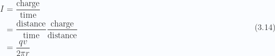
This is an Euclidean space when .

To select from a multivector the grade portion, say we write

The scalar portion of a multivector will be written as

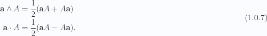
The grade selection operators can be used to define the outer and inner products. For blades , and of grade and respectively, these are

Written out explicitly for odd grade blades (vector, trivector, …), and vector the dot and wedge products are respectively

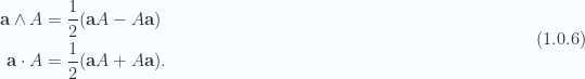
Similarly for even grade blades these are

It will be useful to employ the cyclic scalar reordering identity for the scalar selection operator

For an dimensional vector space, a product of orthonormal (up to a sign) unit vectors is referred to as a pseudoscalar for the space, typically denoted by

The pseudoscalar may commute or anticommute with other blades in the space. We may also form a pseudoscalar for a subspace spanned by vectors by unit scaling the wedge products of those vectors .

Curvilinear coordinates

For our purposes a manifold can be loosely defined as a parameterized surface. For example, a 2D manifold can be considered a surface in an dimensional vector space, parameterized by two variables

Note that the indices here do not represent exponentiation. We can construct a basis for the manifold as

On the manifold we can calculate a reciprocal basis , defined by requiring, at each point on the surface

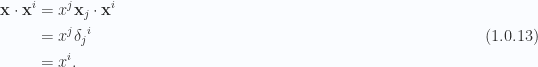
Associated implicitly with this basis is a curvilinear coordinate representation defined by the projection operation

(sums over mixed indices are implied). These coordinates can be calculated by taking dot products with the reciprocal frame vectors

In this document all coordinates are with respect to a specific curvilinear basis, and not with respect to the standard basis or its dual basis unless otherwise noted.

Similar to the usual notation for derivatives with respect to the standard basis coordinates we form a lower index partial derivative operator

so that when the complete vector space is spanned by the gradient has the curvilinear representation

This can be motivated by noting that the directional derivative is defined by

When the basis does not span the space, the projection of the gradient onto the tangent space at the point of evaluation

This is called the vector derivative.

See [6] for a more complete discussion of the gradient and vector derivatives in curvilinear coordinates.

Green’s theorem

Given a two parameter () surface parameterization, the curvilinear coordinate representation of a vector has the form

We assume that the vector space is of dimension two or greater but otherwise unrestricted, and need not have an Euclidean basis. Here denotes the rejection of from the tangent space at the point of evaluation. Green’s theorem relates the integral around a closed curve to an “area” integral on that surface

Theorem 2. Green’s Theorem

Following the arguments used in [7] for Stokes theorem in three dimensions, we first evaluate the loop integral along the differential element of the surface at the point evaluated over the range , as shown in the infinitesimal loop of fig. 1.1.

Fig 1.1. Infinitesimal loop integral

Over the infinitesimal area, the loop integral decomposes into

where the differentials along the curve are

It is assumed that the parameterization change is small enough that this loop integral can be considered planar (regardless of the dimension of the vector space). Making use of the fact that for , the loop integral is

With the distances being infinitesimal, these differences can be rewritten as partial differentials

We can now sum over a larger area as in fig. 1.2

Fig 1.2. Sum of infinitesimal loops

All the opposing oriented loop elements cancel, so the integral around the complete boundary of the surface is given by the area integral of the partials difference.

We will see that Green’s theorem is a special case of the Curl (Stokes) theorem. This observation will also provide a geometric interpretation of the right hand side area integral of thm. 2, and allow for a coordinate free representation.

Special case:

An important special case of Green’s theorem is for a Euclidean two dimensional space where the vector function is

Here Green’s theorem takes the form

Curl theorem, two volume vector field

Having examined the right hand side of thm. 1 for the very simplest geometric object , let’s look at the right hand side, the area integral in more detail. We restrict our attention for now to vectors still defined by eq. 1.19.

First we need to assign a meaning to . By this, we mean the wedge products of the two differential elements. With

that area element is

This is the oriented area element that lies in the tangent plane at the point of evaluation, and has the magnitude of the area of that segment of the surface, as depicted in fig. 1.3.

Fig 1.3. Oriented area element tiling of a surface

Observe that we have no requirement to introduce a normal to the surface to describe the direction of the plane. The wedge product provides the information about the orientation of the place in the space, even when the vector space that our vector lies in has dimension greater than three.

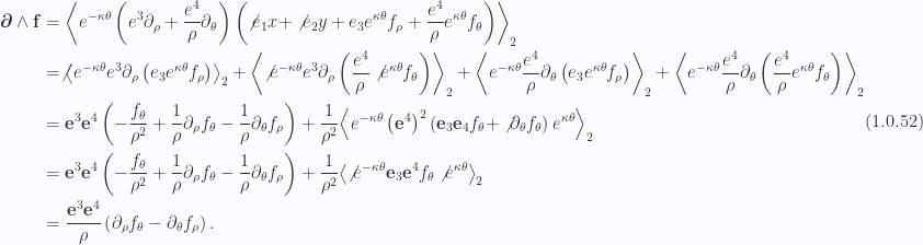
Proceeding with the expansion of the dot product of the area element with the curl, using eq. 1.0.6, eq. 1.0.7, and eq. 1.0.8, and a scalar selection operation, we have

Let’s proceed to expand the inner dot product

The complete curl term is thus

This almost has the form of eq. 1.23, although that is not immediately obvious. Working backwards, using the shorthand , we can show that this coordinate representation can be eliminated

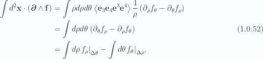
This relates the two parameter surface integral of the curl to the loop integral over its boundary

This is the very simplest special case of Stokes theorem. When written in the general form of Stokes thm. 1

we must remember (the is to remind us of this) that it is implied that both the vector and the differential elements are evaluated on the boundaries of the integration ranges respectively. A more exact statement is

Expanded out in full this is

which can be cross checked against fig. 1.4 to demonstrate that this specifies a clockwise orientation. For the surface with oriented area , the clockwise loop is designated with line elements (1)-(4), we see that the contributions around this loop (in boxes) match eq. 1.0.35.

Fig 1.4. Clockwise loop

Example: Green’s theorem, a 2D Cartesian parameterization for a Euclidean space

For a Cartesian 2D Euclidean parameterization of a vector field and the integration space, Stokes theorem should be equivalent to Green’s theorem eq. 1.0.25. Let’s expand both sides of eq. 1.0.32 independently to verify equality. The parameterization is

Here the dual basis is the basis, and the projection onto the tangent space is just the gradient

The volume element is an area weighted pseudoscalar for the space

and the curl of a vector 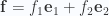is

So, the LHS of Stokes theorem takes the coordinate form

For the RHS, following fig. 1.5, we have

As expected, we can also obtain this by integrating eq. 1.0.38.

Fig 1.5. Euclidean 2D loop

Example: Cylindrical parameterization

Let’s now consider a cylindrical parameterization of a 4D space with Euclidean metric or Minkowski metric . For such a space let’s do a brute force expansion of both sides of Stokes theorem to gain some confidence that all is well.

With , such a space is conveniently parameterized as illustrated in fig. 1.6 as

Fig 1.6. Cylindrical polar parameterization

Note that the Euclidean case where rejection of the non-axial components of expands to

whereas for the Minkowski case where we have a hyperbolic expansion

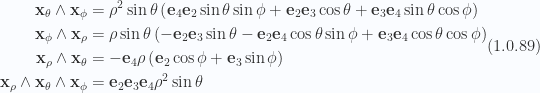
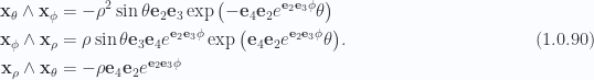
Within such a space consider the surface along , for which the vectors are parameterized by

The tangent space unit vectors are

and

Observe that both of these vectors have their origin at the point of evaluation, and aren’t relative to the absolute origin used to parameterize the complete space.

We wish to compute the volume element for the tangent plane. Noting that and both anticommute with we have for

so

The tangent space volume element is thus

With the tangent plane vectors both perpendicular we don’t need the general lemma 6 to compute the reciprocal basis, but can do so by inspection

and

Observe that the latter depends on the metric signature.

The vector derivative, the projection of the gradient on the tangent space, is

From this we see that acting with the vector derivative on a scalar radial only dependent function is a vector function that has a radial direction, whereas the action of the vector derivative on an azimuthal only dependent function is a vector function that has only an azimuthal direction. The interpretation of the geometric product action of the vector derivative on a vector function is not as simple since the product will be a multivector.

Expanding the curl in coordinates is messier, but yields in the end when tackled with sufficient care

After all this reduction, we can now state in coordinates the LHS of Stokes theorem explicitly

Now compare this to the direct evaluation of the loop integral portion of Stokes theorem. Expressing this using eq. 1.0.34, we have the same result

This example highlights some of the power of Stokes theorem, since the reduction of the volume element differential form was seen to be quite a chore (and easy to make mistakes doing.)

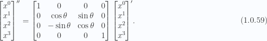
Example: Composition of boost and rotation

Working in a space with basis where and , an active composition of boost and rotation has the form

where is a bivector of a timelike unit vector and perpendicular spacelike unit vector, and is a bivector of two perpendicular spacelike unit vectors. For example, and . For such the respective Lorentz transformation matrices are

and

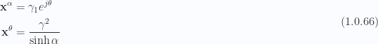
Let’s calculate the tangent space vectors for this parameterization, assuming that the particle is at an initial spacetime position of . That is

To calculate the tangent space vectors for this subspace we note that

and

The tangent space vectors are therefore

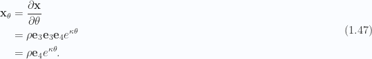
Continuing a specific example where let’s also pick , the spacetime position of a particle at the origin of a frame at that frame’s . The tangent space vectors for the subspace parameterized by this transformation and this initial position is then reduced to

and

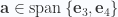
By inspection the dual basis for this parameterization is

So, Stokes theorem, applied to a spacetime vector , for this subspace is

Since the point is to avoid the curl integral, we did not actually have to state it explicitly, nor was there any actual need to calculate the dual basis.

Example: Dual representation in three dimensions

It’s clear that there is a projective nature to the differential form . This projective nature allows us, in three dimensions, to re-express Stokes theorem using the gradient instead of the vector derivative, and to utilize the cross product and a normal direction to the plane.

When we parameterize a normal direction to the tangent space, so that for a 2D tangent space spanned by curvilinear coordinates and the vector is normal to both, we can write our vector as

and express the orientation of the tangent space area element in terms of a pseudoscalar that includes this normal direction

Inserting this into an expansion of the curl form we have

Observe that this last term, the contribution of the component of the gradient perpendicular to the tangent space, has no components

leaving

Now scale the normal vector and its dual to have unit norm as follows

so that for , the volume element can be

This scaling choice is illustrated in fig. 1.7, and represents the “outwards” normal. With such a scaling choice we have

Fig 1.7. Outwards normal

and almost have the desired cross product representation

With the duality identity 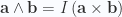, we have the traditional 3D representation of Stokes theorem

Note that the orientation of the loop integral in the traditional statement of the 3D Stokes theorem is counterclockwise instead of clockwise, as written here.

Stokes theorem, three variable volume element parameterization

We can restate the identity of thm. 1 in an equivalent dot product form.

Here , with the implicit assumption that it and the blade that it is dotted with, are both evaluated at the end points of integration variable that has been integrated against.

We’ve seen one specific example of this above in the expansions of eq. 1.28, and eq. 1.29, however, the equivalent result of eq. 1.0.78, somewhat magically, applies to any degree blade and volume element provided the degree of the blade is less than that of the volume element (i.e. ). That magic follows directly from lemma 1.

As an expositional example, consider a three variable volume element parameterization, and a vector blade

It should not be surprising that this has the structure found in the theory of differential forms. Using the differentials for each of the parameterization “directions”, we can write this dot product expansion as

Observe that the sign changes with each element of that is skipped. In differential forms, the wedge product composition of 1-forms is an abstract quantity. Here the differentials are just vectors, and their wedge product represents an oriented volume element. This interpretation is likely available in the theory of differential forms too, but is arguably less obvious.

Digression

As was the case with the loop integral, we expect that the coordinate representation has a representation that can be expressed as a number of antisymmetric terms. A bit of experimentation shows that such a sum, after dropping the parameter space volume element factor, is

To proceed with the integration, we must again consider an infinitesimal volume element, for which the partial can be evaluated as the difference of the endpoints, with all else held constant. For this three variable parameterization, say, , let’s delimit such an infinitesimal volume element by the parameterization ranges , , . The integral is

Extending this over the ranges , , , we have proved Stokes thm. 1 for vectors and a three parameter volume element, provided we have a surface element of the form

where the evaluation of the dot products with are also evaluated at the same points.

Example: Euclidean spherical polar parameterization of 3D subspace

Consider an Euclidean space where a 3D subspace is parameterized using spherical coordinates, as in

The tangent space basis for the subspace situated at some fixed , is easy to calculate, and is found to be

While we can use the general relation of lemma 7 to compute the reciprocal basis. That is

However, a naive attempt at applying this without algebraic software is a route that requires a lot of care, and is easy to make mistakes doing. In this case it is really not necessary since the tangent space basis only requires scaling to orthonormalize, satisfying for

This allows us to read off the dual basis for the tangent volume by inspection

Should we wish to explicitly calculate the curl on the tangent space, we would need these. The area and volume elements are also messy to calculate manually. This expansion can be found in the Mathematica notebook \nbref{sphericalSurfaceAndVolumeElements.nb}, and is

Those area elements have a Geometric algebra factorization that are perhaps useful

One of the beauties of Stokes theorem is that we don’t actually have to calculate the dual basis on the tangent space to proceed with the integration. For that calculation above, where we had a normal tangent basis, I still used software was used as an aid, so it is clear that this can generally get pretty messy.

To apply Stokes theorem to a vector field we can use eq. 1.0.82 to write down the integral directly

Observe that eq. 1.0.90 is a vector valued integral that expands to

This could easily be a difficult integral to evaluate since the vectors evaluated at the endpoints are still functions of two parameters. An easier integral would result from the application of Stokes theorem to a bivector valued field, say , for which we have

There is a geometric interpretation to these oriented area integrals, especially when written out explicitly in terms of the differentials along the parameterization directions. Pulling out a sign explicitly to match the geometry (as we had to also do for the line integrals in the two parameter volume element case), we can write this as

When written out in this differential form, each of the respective area elements is an oriented area along one of the faces of the parameterization volume, much like the line integral that results from a two parameter volume curl integral. This is visualized in fig. 1.8. In this figure, faces (1) and (3) are “top faces”, those with signs matching the tops of the evaluation ranges eq. 1.0.94, whereas face (2) is a bottom face with a sign that is correspondingly reversed.

Fig 1.8. Boundary faces of a spherical parameterization region

Example: Minkowski hyperbolic-spherical polar parameterization of 3D subspace

Working with a three parameter volume element in a Minkowski space does not change much. For example in a 4D space with , we can employ a hyperbolic-spherical parameterization similar to that used above for the 4D Euclidean space

This has tangent space basis elements

This is a normal basis, but again not orthonormal. Specifically, for we have

where we see that the radial vector is timelike. We can form the dual basis again by inspection

The area elements are

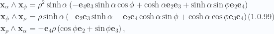
or

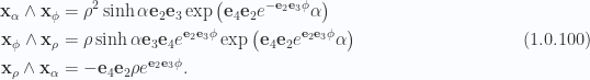
The volume element also reduces nicely, and is

The area and volume element reductions were once again messy, done in software using \nbref{sphericalSurfaceAndVolumeElementsMinkowski.nb}. However, we really only need eq. 1.0.96 to perform the Stokes integration.

Stokes theorem, four variable volume element parameterization

Volume elements for up to four parameters are likely of physical interest, with the four volume elements of interest for relativistic physics in spaces. For example, we may wish to use a parameterization , with a four volume

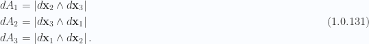
We follow the same procedure to calculate the corresponding boundary surface “area” element (with dimensions of volume in this case). This is

Our boundary value surface element is therefore

where it is implied that this (and the dot products with ) are evaluated on the boundaries of the integration ranges of the omitted index. This same boundary form can be used for vector, bivector and trivector variations of Stokes theorem.

Duality and its relation to the pseudoscalar.

Looking to eq. 1.0.181 of lemma 6, and scaling the wedge product by its absolute magnitude, we can express duality using that scaled bivector as a pseudoscalar for the plane that spans . Let’s introduce a subscript notation for such scaled blades

This allows us to express the unit vector in the direction of as

Following the pattern of eq. 1.0.181, it is clear how to express the dual vectors for higher dimensional subspaces. For example

or for the unit vector in the direction of ,

Divergence theorem.

When the curl integral is a scalar result we are able to apply duality relationships to obtain the divergence theorem for the corresponding space. We will be able to show that a relationship of the following form holds

Here is a vector, is normal to the boundary surface, and is the area of this bounding surface element. We wish to quantify these more precisely, especially because the orientation of the normal vectors are metric dependent. Working a few specific examples will show the pattern nicely, but it is helpful to first consider some aspects of the general case.

First note that, for a scalar Stokes integral we are integrating the vector derivative curl of a blade over a k-parameter volume element. Because the dimension of the space matches the number of parameters, the projection of the gradient onto the tangent space is exactly that gradient

Multiplication of by the pseudoscalar will always produce a vector. With the introduction of such a dual vector, as in

Stokes theorem takes the form

or

where we will see that the vector can roughly be characterized as a normal to the boundary surface. Using primes to indicate the scope of the action of the gradient, cyclic permutation within the scalar selection operator can be used to factor out the pseudoscalar

The second last step uses lemma 8, and the last writes , where we have assumed (without loss of generality) that has the same orientation as the pseudoscalar for the space. We also assume that the parameterization is non-degenerate over the integration volume (i.e. no ), so the sign of this product cannot change.

Let’s now return to the normal vector . With (the indexed differential omitted), and , we have

We’ve seen in eq. 1.0.106 and lemma 7 that the dual of vector with respect to the unit pseudoscalar in a subspace spanned by is

or

This allows us to write

where , and is the area of the boundary area element normal to . Note that the term will now cancel cleanly from both sides of the divergence equation, taking both the metric and the orientation specific dependencies with it.

This leaves us with

To spell out the details, we have to be very careful with the signs. However, that is a job best left for specific examples.

Example: 2D divergence theorem

Let’s start back at

On the left our integral can be rewritten as

where and we pick the pseudoscalar with the same orientation as the volume (area in this case) element .

For the boundary form we have

The duality relations for the tangent space are

or

Back substitution into the line element gives

Writing (no sum) , we have

This provides us a divergence and normal relationship, with terms on each side that can be canceled. Restoring explicit range evaluation, that is

Let’s consider this graphically for an Euclidean metric as illustrated in fig. 1.9.

Fig 1.9. Normals on area element

We see that

1. along the outwards normal is ,
2. along the outwards normal is ,
3. along the outwards normal is , and
4. along the outwards normal is .

Writing that outwards normal as , we have

Note that we can use the same algebraic notion of outward normal for non-Euclidean spaces, although cannot expect the geometry to look anything like that of the figure.

Example: 3D divergence theorem

As with the 2D example, let’s start back with

In a 3D space, the pseudoscalar commutes with all grades, so we have

where , and we have used a pseudoscalar with the same orientation as the volume element

In the boundary integral our dual two form is

where , and

Observe that we can do a cyclic permutation of a 3 blade without any change of sign, for example

Because of this we can write the dual two form as we expressed the normals in lemma 7

We can now state the 3D divergence theorem, canceling out the metric and orientation dependent term on both sides

where (sums implied)

and

The outwards normals at the upper integration ranges of a three parameter surface are depicted in fig. 1.10.

Fig 1.10. Outwards normals on volume at upper integration ranges.

This sign alternation originates with the two form elements from the Stokes boundary integral, which were explicitly evaluated at the endpoints of the integral. That is, for ,

In the context of the divergence theorem, this means that we are implicitly requiring the dot products to be evaluated specifically at the end points of the integration where , accounting for the alternation of sign required to describe the normals as uniformly outwards.

Example: 4D divergence theorem

Applying Stokes theorem to a trivector in the 4D case we find

Here the pseudoscalar has been picked to have the same orientation as the hypervolume element . Writing the dual of the three form is

Here, we’ve written

Observe that the dual representation nicely removes the alternation of sign that we had in the Stokes theorem boundary integral, since each alternation of the wedged vectors in the pseudoscalar changes the sign once.

As before, we define the outwards normals as on the upper and lower integration ranges respectively. The scalar area elements on these faces can be written in a dual form

so that the 4D divergence theorem looks just like the 2D and 3D cases

Here we define the volume scaled normal as

As before, we have made use of the implicit fact that the three form (and it’s dot product with ) was evaluated on the boundaries of the integration region, with a toggling of sign on the lower limit of that evaluation that is now reflected in what we have defined as the outwards normal.

We also obtain explicit instructions from this formalism how to compute the “outwards” normal for this surface in a 4D space (unit scaling of the dual basis elements), something that we cannot compute using any sort of geometrical intuition. For free we’ve obtained a result that applies to both Euclidean and Minkowski (or other non-Euclidean) spaces.

Volume integral coordinate representations

It may be useful to formulate the curl integrals in tensor form. For vectors , and bivectors , the coordinate representations of those differential forms (\cref{pr:stokesTheoremGeometricAlgebraII:1}) are

Here the bivector and trivector is expressed in terms of their curvilinear components on the tangent space

where

For the trivector components are also antisymmetric, changing sign with any interchange of indices.

Note that eq. 1.0.144d and eq. 1.0.144f appear much different on the surface, but both have the same structure. This can be seen by writing for former as

In both of these we have an alternation of sign, where the tensor index skips one of the volume element indices is sequence. We’ve seen in the 4D divergence theorem that this alternation of sign can be related to a duality transformation.

In integral form (no sum over indexes in terms), these are

Of these, I suspect that only eq. 1.0.148a and eq. 1.0.148d are of use.

Final remarks

Because we have used curvilinear coordinates from the get go, we have arrived naturally at a formulation that works for both Euclidean and non-Euclidean geometries, and have demonstrated that Stokes (and the divergence theorem) holds regardless of the geometry or the parameterization. We also know explicitly how to formulate both theorems for any parameterization that we choose, something much more valuable than knowledge that this is possible.

For the divergence theorem we have introduced the concept of outwards normal (for example in 3D, eq. 1.0.136), which still holds for non-Euclidean geometries. We may not be able to form intuitive geometrical interpretations for these normals, but do have an algebraic description of them.

Appendix

Problems

Question: Expand volume elements in coordinates

Show that the coordinate representation for the volume element dotted with the curl can be represented as a sum of antisymmetric terms. That is

• (a)Prove eq. 1.0.144a
• (b)Prove eq. 1.0.144b
• (c)Prove eq. 1.0.144c
• (d)Prove eq. 1.0.144d
• (e)Prove eq. 1.0.144e
• (f)Prove eq. 1.0.144f

Answer

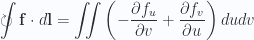
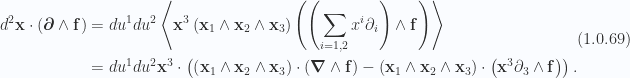
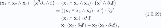
(a) Two parameter volume, curl of vector

(b) Three parameter volume, curl of vector

(c) Four parameter volume, curl of vector

(d) Three parameter volume, curl of bivector

(e) Four parameter volume, curl of bivector

To start, we require lemma 3. For convenience lets also write our wedge products as a single indexed quantity, as in for . The expansion is

This last step uses an intermediate result from the eq. 1.0.152 expansion above, since each of the four terms has the same structure we have previously observed.

(f) Four parameter volume, curl of trivector

Using the shorthand again, the initial expansion gives

Applying lemma 4 to expand the inner products within the braces we have

We can cancel those last terms using lemma 5. Using the same reverse chain rule expansion once more we have

or

The final result follows after permuting the indices slightly.

Some helpful identities

Lemma 1. Distribution of inner products

Given two blades with grades subject to , and a vector , the inner product distributes according to

This will allow us, for example, to expand a general inner product of the form .

The proof is straightforward, but also mechanical. Start by expanding the wedge and dot products within a grade selection operator

Solving for in

we have

The last term above is zero since we are selecting the grade element of a multivector with grades and , which has no terms for . Now we can expand the multivector product, for

The latter multivector (with the wedge product factor) above has grades and , so this selection operator finds nothing. This leaves

The first dot products term has grade and is selected, whereas the wedge term has grade (for ).

Lemma 2. Distribution of two bivectors

For vectors , , and bivector , we have

Proof follows by applying the scalar selection operator, expanding the wedge product within it, and eliminating any of the terms that cannot contribute grade zero values

Lemma 3. Inner product of trivector with bivector

Given a bivector , and trivector where and are vectors, the inner product is

This is also problem 1.1(c) from Exercises 2.1 in [3], and submits to a dumb expansion in successive dot products with a final regrouping. With

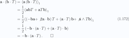
Lemma 4. Distribution of two trivectors

Given a trivector and three vectors , and , the entire inner product can be expanded in terms of any successive set inner products, subject to change of sign with interchange of any two adjacent vectors within the dot product sequence

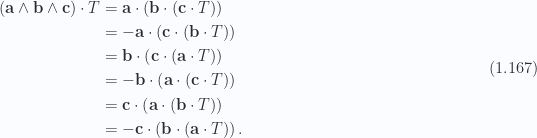
To show this, we first expand within a scalar selection operator

Now consider any single term from the scalar selection, such as the first. This can be reordered using the vector dot product identity

The vector-trivector product in the latter grade selection operation above contributes only bivector and quadvector terms, thus contributing nothing. This can be repeated, showing that

Substituting this back into eq. 1.0.168 proves lemma 4.

Lemma 5. Permutation of two successive dot products with trivector

Given a trivector and two vectors and , alternating the order of the dot products changes the sign

This and lemma 4 are clearly examples of a more general identity, but I’ll not try to prove that here. To show this one, we have

Cancellation of terms above was because they could not contribute to a grade one selection. We also employed the relation 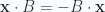for bivector and vector .

Lemma 6. Duality in a plane

For a vector , and a plane containing and , the dual of this vector with respect to this plane is

Satisfying

and

To demonstrate, we start with the expansion of

Dotting with we have

but dotting with yields zero

To complete the proof, we note that the product in eq. 1.177 is just the wedge squared

This duality relation can be recast with a linear denominator

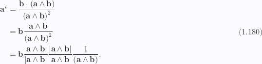
or

We can use this form after scaling it appropriately to express duality in terms of the pseudoscalar.

Lemma 7. Dual vector in a three vector subspace

In the subspace spanned by , the dual of is

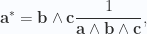
Consider the dot product of with .

The canceled term is eliminated since it is the product of a vector and trivector producing no scalar term. Substituting , and noting that , we have

Lemma 8. Pseudoscalar selection

For grade blade (i.e. a pseudoscalar), and vectors , the grade selection of this blade sandwiched between the vectors is

To show this, we have to consider even and odd grades separately. First for even we have

or

Similarly for odd , we have

or

Adjusting for the signs completes the proof.

References

[1] John Denker. Magnetic field for a straight wire., 2014. URL http://www.av8n.com/physics/straight-wire.pdf. [Online; accessed 11-May-2014].

[2] H. Flanders. Differential Forms With Applications to the Physical Sciences. Courier Dover Publications, 1989.

[3] D. Hestenes. New Foundations for Classical Mechanics. Kluwer Academic Publishers, 1999.

[4] Peeter Joot. Collection of old notes on Stokes theorem in Geometric algebra, 2014. URL https://sites.google.com/site/peeterjoot3/math2014/bigCollectionOfPartiallyIncorrectStokesTheoremMusings.pdf.

[5] Peeter Joot. Synposis of old notes on Stokes theorem in Geometric algebra, 2014. URL https://sites.google.com/site/peeterjoot3/math2014/synopsisOfBigCollectionOfPartiallyIncorrectStokesTheoremMusings.pdf.

[6] A. Macdonald. Vector and Geometric Calculus. CreateSpace Independent Publishing Platform, 2012.

[7] M. Schwartz. Principles of Electrodynamics. Dover Publications, 1987.

[8] Michael Spivak. Calculus on manifolds, volume 1. Benjamin New York, 1965.

Geometric Algebra. The very quickest introduction.

[Click here for a PDF of this post with nicer formatting.]

Motivation.

An attempt to make a relatively concise introduction to Geometric (or Clifford) Algebra. Much more complete introductions to the subject can be found in [1], [2], and [3].

Axioms

We have a couple basic principles upon which the algebra is based

1. Vectors can be multiplied.
2. The square of a vector is the (squared) length of that vector (with appropriate generalizations for non-Euclidean metrics).
3. Vector products are associative (but not necessarily commutative).

That’s really all there is to it, and the rest, paraphrasing Feynman, can be figured out by anybody sufficiently clever.

By example. The 2D case.

Consider a 2D Euclidean space, and the product of two vectors and in that space. Utilizing a standard orthonormal basis we can write

and let’s write out the product of these two vectors , not yet knowing what we will end up with. That is

From axiom 2 we have , so we have

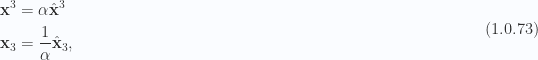
We’ve multiplied two vectors and ended up with a scalar component (and recognize that this part of the vector product is the dot product), and a component that is a “something else”. We’ll call this something else a bivector, and see that it is characterized by a product of non-colinear vectors. These products and are in fact related, and we can see that by looking at the case of . For that we have

Since axiom (2) requires our vectors square to equal its (squared) length, we must then have

or

We see that Euclidean orthonormal vectors anticommute. What we can see with some additional study is that any colinear vectors commute, and in Euclidean spaces (of any dimension) vectors that are normal to each other anticommute (this can also be taken as a definition of normal).

We can now return to our product of two vectors 3.3 and simplify it slightly

The product of two vectors in 2D is seen here to have one scalar component, and one bivector component (an irreducible product of two normal vectors). Observe the symmetric and antisymmetric split of the scalar and bivector components above. This symmetry and antisymmetry can be made explicit, introducing dot and wedge product notation respectively

so that the vector product can be written as

Pseudoscalar

In many contexts it is useful to introduce an ordered product of all the unit vectors for the space is called the pseudoscalar. In our 2D case this is

a quantity that we find behaves like the complex imaginary. That can be shown by considering its square

Here the anticommutation of normal vectors property has been used, as well as (for the first time) the associative multiplication axiom.

In a 3D context, you’ll see the pseudoscalar in many places (expressing the normals to planes for example). It also shows up in a number of fundamental relationships. For example, if one writes

for the 3D pseudoscalar, then it’s also possible to show

something that will be familiar to the student of QM, where we see this in the context of Pauli matrices. The Pauli matrices also encode a Clifford algebraic structure, but we do not need an explicit matrix representation to do so.

Rotations

Very much like complex numbers we can utilize exponentials to perform rotations. Rotating in a sense from to , can be expressed as

More generally, even in N dimensional Euclidean spaces, if is a vector in a plane, and and are perpendicular unit vectors in that plane, then the rotation through angle is given by

This is illustrated in figure (1).

Plane rotation.

 

Notice that we have expressed the rotation here without utilizing a normal direction for the plane. The sense of the rotation is encoded by the bivector that describes the plane and the orientation of the rotation (or by duality the direction of the normal in a 3D space). By avoiding a requirement to encode the rotation using a normal to the plane we have an method of expressing the rotation that works not only in 3D spaces, but also in 2D and greater than 3D spaces, something that isn’t possible when we restrict ourselves to traditional vector algebra (where quantities like the cross product can’t be defined in a 2D or 4D space, despite the fact that things they may represent, like torque are planar phenomena that do not have any intrinsic requirement for a normal that falls out of the plane.).

When does not lie in the plane spanned by the vectors and , as in figure (2), we must express the rotations differently. A rotation then takes the form

3D rotation.

 

In the 2D case, and when the vector lies in the plane this reduces to the one sided complex exponential operator used above. We see these types of paired half angle rotations in QM, and they are also used extensively in computer graphics under the guise of quaternions.

References

[1] L. Dorst, D. Fontijne, and S. Mann. Geometric Algebra for Computer Science. Morgan Kaufmann, San Francisco, 2007.

[2] C. Doran and A.N. Lasenby. Geometric algebra for physicists. Cambridge University Press New York, Cambridge, UK, 1st edition, 2003.

[3] D. Hestenes. New Foundations for Classical Mechanics. Kluwer Academic Publishers, 1999.

PHY456H1F: Quantum Mechanics II. Lecture 15 (Taught by Prof J.E. Sipe). Rotation operator in spin space

[Click here for a PDF of this post with nicer formatting and figures if the post had any (especially if my latex to wordpress script has left FORMULA DOES NOT PARSE errors.)]

Disclaimer.

Peeter’s lecture notes from class. May not be entirely coherent.

Rotation operator in spin space.

We can formally expand our rotation operator in Taylor series

or

where we’ve used the fact that .

So our representation of the spin operator is

Note that, in particular,

This “rotates” the ket, but introduces a phase factor.

Can do this in general for other degrees of spin, for .

Unfortunate interjection by me

I mentioned the half angle rotation operator that requires a half angle operator sandwich. Prof. Sipe thought I might be talking about a Heisenberg picture representation, where we have something like this in expectation values

so that

However, what I was referring to, was that a general rotation of a vector in a Pauli matrix basis

can be expressed by sandwiching the Pauli vector representation by two half angle rotation operators like our spin 1/2 operators from class today

where and are two non-colinear orthogonal unit vectors that define the oriented plane that we are rotating in.

For example, rotating in the plane, with and , we have

Observe that these exponentials commute with , leaving

yielding our usual coordinate rotation matrix. Expressed in terms of a unit normal to that plane, we form the normal by multiplication with the unit spatial volume element . For example:

and can in general write a spatial rotation in a Pauli basis representation as a sandwich of half angle rotation matrix exponentials

when we get the complex-number like single sided exponential rotation exponentials (since commutes with in that case)

I believe it was pointed out in one of [1] or [2] that rotations expressed in terms of half angle Pauli matrices has caused some confusion to students of quantum mechanics, because this “rotation” only generates half of the full spatial rotation. It was argued that this sort of confusion can be avoided if one observes that these half angle rotations exponentials are exactly what we require for general spatial rotations, and that a pair of half angle operators are required to produce a full spatial rotation.

The book [1] takes this a lot further, and produces a formulation of spin operators that is devoid of the normal scalar imaginary (using the Clifford algebra spatial unit volume element instead), and also does not assume a specific matrix representation of the spin operators. They argue that this leads to some subtleties associated with interpretation, but at the time I was attempting to read that text I did know enough QM to appreciate what they were doing, and haven’t had time to attempt a new study of that content.

Spin dynamics

At least classically, the angular momentum of charged objects is associated with a magnetic moment as illustrated in figure (\ref{fig:qmTwoL15:qmTwoL15fig1})

\begin{figure}[htp]
\centering
\includegraphics[totalheight=0.2\textheight]{qmTwoL15fig1}
\caption{Magnetic moment due to steady state current}
\end{figure}

In our scheme, following the (cgs?) text conventions of [3], where the and have the same units, we write

For a charge moving in a circle as in figure (\ref{fig:qmTwoL15:qmTwoL15fig2})
\begin{figure}[htp]
\centering
\includegraphics[totalheight=0.2\textheight]{qmTwoL15fig2}
\caption{Charge moving in circle.}
\end{figure}

so the magnetic moment is

Here is the gyromagnetic ratio

Recall that we have a torque, as shown in figure (\ref{fig:qmTwoL15:qmTwoL15fig3})
\begin{figure}[htp]
\centering
\includegraphics[totalheight=0.2\textheight]{qmTwoL15fig3}
\caption{Induced torque in the presence of a magnetic field.}
\end{figure}

tending to line up with . The energy is then

Also recall that this torque leads to precession as shown in figure (\ref{fig:qmTwoL15:qmTwoL15fig4})

\begin{figure}[htp]
\centering
\includegraphics[totalheight=0.2\textheight]{qmTwoL15fig4}
\caption{Precession due to torque.}
\end{figure}

with precession frequency

For a current due to a moving electron

where we are, here, writing for charge on the electron .

Question: steady state currents only?. Yes, this is only true for steady state currents.

For the translational motion of an electron, even if it is not moving in a steady way, regardless of it’s dynamics

Now, back to quantum mechanics, we turn into a dipole moment operator and is “promoted” to an angular momentum operator.

What about the “spin”?

Perhaps

we write this as

so that

Experimentally, one finds to very good approximation

There was a lot of trouble with this in early quantum mechanics where people got things wrong, and canceled the wrong factors of .

In fact, Dirac’s relativistic theory for the electron predicts .

When this is measured experimentally, one does not get exactly , and a theory that also incorporates photon creation and destruction and the interaction with the electron with such (virtual) photons. We get

Richard Feynman compared the precision of quantum mechanics, referring to this measurement, “to predicting a distance as great as the width of North America to an accuracy of one human hair’s breadth”.

References

[1] C. Doran and A.N. Lasenby. Geometric algebra for physicists. Cambridge University Press New York, Cambridge, UK, 1st edition, 2003.

[2] D. Hestenes. New Foundations for Classical Mechanics. Kluwer Academic Publishers, 1999.

[3] BR Desai. Quantum mechanics with basic field theory. Cambridge University Press, 2009.

new version of geometric algebra notes compilation

Newly added to the compilation (version 10) since last update are:

April 30, 2011 A cylindrical Lienard-Wiechert potential calculation using multivector matrix products.

Dec 27, 2010 Vector form of Julia fractal.

Some typos are probably fixed too.

Changelog for version 9 was here.

PHY456H1F: Quantum Mechanics II. Lecture 6 (Taught by Prof J.E. Sipe). Interaction picture.

[Click here for a PDF of this post with nicer formatting (especially if my latex to wordpress script has left FORMULA DOES NOT PARSE errors.)]

Disclaimer.

Peeter’s lecture notes from class. May not be entirely coherent.

Interaction picture.

Recap.

Recall our table comparing our two interaction pictures

A motivating example.

While fundamental Hamiltonians are independent of time, in a number of common cases, we can form approximate Hamiltonians that are time dependent. One such example is that of Coulomb excitations of an atom, as covered in section 18.3 of the text [1], and shown in figure (\ref{fig:qmTwoL6fig1}).

\begin{figure}[htp]
\centering
\includegraphics[totalheight=0.4\textheight]{qmTwoL6fig1}
\caption{Coulomb interaction of a nucleus and heavy atom.}
\end{figure}

We consider the interaction of a nucleus with a neutral atom, heavy enough that it can be considered classically. From the atoms point of view, the effects of the heavy nucleus barreling by can be described using a time dependent Hamiltonian. For the atom, that interaction Hamiltonian is

Here and is the position vector for the heavy nucleus, and is the position to each charge within the atom, where ranges over all the internal charges, positive and negative, within the atom.

Placing the origin close to the atom, we can write this interaction Hamiltonian as

The first term vanishes because the total charge in our neutral atom is zero. This leaves us with

where is the electric field at the origin due to the nucleus.

Introducing a dipole moment operator for the atom

the interaction takes the form

Here we have a quantum mechanical operator, and a classical field taken together. This sort of dipole interaction also occurs when we treat a atom placed into an electromagnetic field, treated classically as depicted in figure (\ref{fig:qmTwoL6fig2})

\begin{figure}[htp]
\centering
\includegraphics[totalheight=0.4\textheight]{qmTwoL6fig2}
\caption{atom in a field}
\end{figure}

In the figure, we can use the dipole interaction, provided , where is the “width” of the atom.

Because it is great for examples, we will see this dipole interaction a lot.

The interaction picture.

Having talked about both the Schr\”{o}dinger and Heisenberg pictures, we can now move on to describe a hybrid, one where our Hamiltonian has been split into static and time dependent parts

We will formulate an approach for dealing with problems of this sort called the interaction picture.

This is also covered in section 3.3 of the text, albeit in a much harder to understand fashion (the text appears to try to not pull the result from a magic hat, but the steps to get to the end result are messy). It would probably have been nicer to see it this way instead.

In the Schr\”{o}dinger picture our dynamics have the form

How about the Heisenberg picture? We look for a solution

We want to find this operator that evolves the state from the state as some initial time , to the arbitrary later state found at time . Plugging in we have

This has to hold for all , and we can equivalently seek a solution of the operator equation

where

the identity for the Hilbert space.

Suppose that was independent of time. We could find that

If depends on time could you guess that

holds? No. This may be true when is a number, but when it is an operator, the Hamiltonian does not necessarily commute with itself at different times

So this is wrong in general. As an aside, for numbers, 2.13 can be verified easily. We have

Expectations

Suppose that we do find . Then our expectation takes the form

Put

and form

so that our expectation has the familiar representations

New strategy. Interaction picture.

Let’s define

or

Let’s see how this works. We have

Define

so that our operator equation takes the form

Note that we also have the required identity at the initial time

Without requiring us to actually find all of the dynamics of the time dependent interaction are now embedded in our operator equation for , with all of the simple interaction related to the non time dependent portions of the Hamiltonian left separate.

Connection with the Schr\”{o}dinger picture.

In the Schr\”{o}dinger picture we have

With a definition of the interaction picture ket as

the Schr\”{o}dinger picture is then related to the interaction picture by

Also, by multiplying 2.22 by our Schr\”{o}dinger ket, we remove the last vestiges of and from the dynamical equation for our time dependent interaction

Interaction picture expectation.

Inverting 2.25, we can form an operator expectation, and relate it the interaction and Schr\”{o}dinger pictures

With a definition

we have

As before, the time evolution of our interaction picture operator, can be found by taking derivatives of 2.28, for which we find

Summarizing the interaction picture.

Given

and initial time states

we have

where

and

or

Our interaction picture Hamiltonian is

and for Schr\”{o}dinger operators, independent of time, we have the dynamical equation

Justifying the Taylor expansion above (not class notes).

Multivariable Taylor series

As outlined in section 2.8 () of [2], we want to derive the multi-variable Taylor expansion for a scalar valued function of some number of variables

consider the displacement operation applied to the vector argument

We can Taylor expand a single variable function without any trouble, so introduce

where

We have

so that

The multivariable Taylor series now becomes a plain old application of the chain rule, where we have to evaluate

so that

Assuming an Euclidean space we can write this in the notationally more pleasant fashion using a gradient operator for the space

To handle the higher order terms, we repeat the chain rule application, yielding for example

Thus the Taylor series associated with a vector displacement takes the tidy form

Even more fancy, we can form the operator equation

Here a dummy variable has been retained as an instruction not to differentiate the part of the directional derivative in any repeated applications of the operator.

That notational cludge can be removed by swapping and

where .

Having derived this (or for those with lesser degrees of amnesia, recall it), we can see that 2.2 was a direct application of this, retaining no second order or higher terms.

Our expression used in the interaction Hamiltonian discussion was

which we can see has the same structure as above with some variable substitutions. Evaluating it we have

and at we have

We see in this direction derivative produces the classical electric Coulomb field expression for an electrostatic distribution, once we take the and multiply it with the factor.

With algebra.

A different way to justify the expansion of 2.2 is to consider a Clifford algebra factorization (following notation from [3]) of the absolute vector difference, where is considered small.

Neglecting the term, we can then Taylor series expand this scalar expression

Observe this is what was found with the multivariable Taylor series expansion too.

References

[1] BR Desai. Quantum mechanics with basic field theory. Cambridge University Press, 2009.

[2] D. Hestenes. New Foundations for Classical Mechanics. Kluwer Academic Publishers, 1999.

[3] C. Doran and A.N. Lasenby. Geometric algebra for physicists. Cambridge University Press New York, Cambridge, UK, 1st edition, 2003.

PHY450HS1: Relativistic electrodynamics: some exam reflection.

[Click here for a PDF of this post with nicer formatting (especially if my latex to wordpress script has left FORMULA DOES NOT PARSE errors.)]

Charged particle in a circle.

From the 2008 PHY353 exam, given a particle of charge moving in a circle of radius at constant angular frequency .

\begin{itemize}
\item Find the Lienard-Wiechert potentials for points on the z-axis.
\item Find the electric and magnetic fields at the center.
\end{itemize}

When I tried this I did it for points not just on the z-axis. It turns out that we also got this question on the exam (but stated slightly differently). Since I’ll not get to see my exam solution again, let’s work through this at a leisurely rate, and see if things look right. The problem as stated in this old practice exam is easier since it doesn’t say to calculate the fields from the four potentials, so there was nothing preventing one from just grinding away and plugging stuff into the Lienard-Wiechert equations for the fields (as I did when I tried it for practice).

The potentials.

Let’s set up our coordinate system in cylindrical coordinates. For the charged particle and the point that we measure the field, with

Here I’m using the geometric product of vectors (if that’s unfamiliar then just substitute

We can do that since the Pauli matrices also have the same semantics (with a small difference since the geometric square of a unit vector is defined as the unit scalar, whereas the Pauli matrix square is the identity matrix). The semantics we require of this vector product are just and for any .

I’ll also be loose with notation and use to select the scalar part of a multivector (or with the Pauli matrices, the portion proportional to the identity matrix).

Our task is to compute the Lienard-Wiechert potentials. Those are

where

We’ll need (eventually)

and also need our retarded distance vector

From this we have

So

Next we need

So we have

Writing , and having a peek back at 1.4, our potentials are now solved for

The caveat is that is only specified implicitly, according to

There doesn’t appear to be much hope of solving for explicitly in closed form.

General fields for this system.

With

the fields are

In there we have

and

Writing this out in coordinates isn’t particularly illuminating, but can be done for completeness without too much trouble

In one sense the problem could be considered solved, since we have all the pieces of the puzzle. The outstanding question is whether or not the resulting mess can be simplified at all. Let’s see if the cross product reduces at all. Using

Perhaps one or more of these dot products can be simplified? One of them does reduce nicely

Putting this cross product back together we have

Writing

this can be grouped into similar terms

The electric field pieces can now be collected. Not expanding out the from 1.14, this is

Along the z-axis where what do we have?

The magnetic term here looks like it can be reduced a bit.

An approximation near the center.

Unlike the old exam I did, where it didn’t specify that the potentials had to be used to calculate the fields, and the problem was reduced to one of algebraic manipulation, our exam explicitly asked for the potentials to be used to calculate the fields.

There was also the restriction to compute them near the center. Setting so that we are looking only near the z-axis, we have

Now we are set to calculate the electric and magnetic fields directly from these. Observe that we have a spatial dependence in due to the quantities and that will have an effect when we operate with the gradient.

In the exam I’d asked Simon (our TA) if this question was asking for the fields at the origin (ie: in the plane of the charge’s motion in the center) or along the z-axis. He said in the plane. That would simplify things, but perhaps too much since becomes constant (in my exam attempt I somehow fudged this to get what I wanted for the case, but that must have been wrong, and was the result of rushed work).

Let’s now proceed with the field calculation from these potentials

For the electric field we need

and

Putting these together, our electric field near the z-axis is

(another mistake I made on the exam, since I somehow fooled myself into forcing what I knew had to be in the gradient term, despite having essentially a constant scalar potential (having taken )).

What do we get for the magnetic field. In that case we have

For the direction vectors in the cross products above we have

and

Putting everything, and summarizing results for the fields, we have

The electric field expression above compares well to 1.29. We have the Coulomb term and the radiation term. It is harder to compare the magnetic field to the exact result 1.30 since I did not expand that out.

FIXME: A question to consider. If all this worked should we not also get

However, if I do this check I get

Collision of photon and electron.

I made a dumb error on the exam on this one. I setup the four momentum conservation statement, but then didn’t multiply out the cross terms properly. This led me to incorrectly assume that I had to try doing this the hard way (something akin to what I did on the midterm). Simon later told us in the tutorial the simple way, and that’s all we needed here too. Here’s the setup.

An electron at rest initially has four momentum

where the incoming photon has four momentum

After the collision our electron has some velocity so its four momentum becomes (say)

and our new photon, going off on an angle relative to has four momentum

Our conservation relationship is thus

I squared both sides, but dropped my cross terms, which was just plain wrong, and costly for both time and effort on the exam. What I should have done was just

and then square this (really making contractions of the form ). That gives (and this time keeping my cross terms)

Rearranging a bit we have

or

Pion decay.

The problem above is very much like a midterm problem we had, so there was no justifiable excuse for messing up on it. That midterm problem was to consider the split of a pion at rest into a neutrino (massless) and a muon, and to calculate the energy of the muon. That one also follows the same pattern, a calculation of four momentum conservation, say

Here is the frequency of the massless neutrino. The massless nature is encoded by a four momentum that squares to zero, which follows from .

When I did this problem on the midterm, I perversely put in a scattering angle, instead of recognizing that the particles must scatter at 180 degree directions since spatial momentum components must also be preserved. This and the combination of trying to work in spatial quantities led to a mess and I didn’t get the end result in anything that could be considered tidy.

The simple way to do this is to just rearrange to put the null vector on one side, and then square. This gives us

A final re-arrangement gives us the muon energy

Fourier transform solutions and associated energy and momentum for the homogeneous Maxwell equation. (rework once more)

[Click here for a PDF of this post with nicer formatting]. Note that this PDF file is formatted in a wide-for-screen layout that is probably not good for printing.

These notes build on and replace those formerly posted in Energy and momentum for assumed Fourier transform solutions to the homogeneous Maxwell equation.

Motivation and notation.

In Electrodynamic field energy for vacuum (reworked) [1], building on Energy and momentum for Complex electric and magnetic field phasors [2], a derivation for the energy and momentum density was derived for an assumed Fourier series solution to the homogeneous Maxwell’s equation. Here we move to the continuous case examining Fourier transform solutions and the associated energy and momentum density.

A complex (phasor) representation is implied, so taking real parts when all is said and done is required of the fields. For the energy momentum tensor the Geometric Algebra form, modified for complex fields, is used

The assumed four vector potential will be written

Subject to the requirement that is a solution of Maxwell’s equation

To avoid latex hell, no special notation will be used for the Fourier coefficients,

When convenient and unambiguous, this dependence will be implied.

Having picked a time and space representation for the field, it will be natural to express both the four potential and the gradient as scalar plus spatial vector, instead of using the Dirac basis. For the gradient this is

and for the four potential (or the Fourier transform functions), this is

Setup

The field bivector is required for the energy momentum tensor. This is

This last term is a spatial curl and the field is then

Applied to the Fourier representation this is

It is only the real parts of this that we are actually interested in, unless physical meaning can be assigned to the complete complex vector field.

Constraints supplied by Maxwell’s equation.

A Fourier transform solution of Maxwell’s vacuum equation has been assumed. Having expressed the Faraday bivector in terms of spatial vector quantities, it is more convenient to do this back substitution into after pre-multiplying Maxwell’s equation by , namely

Applied to the spatially decomposed field as specified in (2.7), this is

All grades of this equation must simultaneously equal zero, and the bivector grades have canceled (assuming commuting space and time partials), leaving two equations of constraint for the system

It is immediately evident that a gauge transformation could be immediately helpful to simplify things. In [3] the gauge choice is used. From (3.11) this implies that . Bohm argues that for this current and charge free case this implies , but he also has a periodicity constraint. Without a periodicity constraint it is easy to manufacture non-zero counterexamples. One is a linear function in the space and time coordinates

This is a valid scalar potential provided that the wave equation for the vector potential is also a solution. We can however, force by making the transformation , which in non-covariant notation is

If the transformed field can be forced to zero, then the complexity of the associated Maxwell equations are reduced. In particular, antidifferentiation of , yields

Dropping primes, the transformed Maxwell equations now take the form

There are two classes of solutions that stand out for these equations. If the vector potential is constant in time , Maxwell’s equations are reduced to the single equation

Observe that a gradient can be factored out of this equation

The solutions are then those s that satisfy both

In particular any non-time dependent potential with constant curl provides a solution to Maxwell’s equations. There may be other solutions to (3.19) too that are more general. Returning to (3.17) a second way to satisfy these equations stands out. Instead of requiring of constant curl, constant divergence with respect to the time partial eliminates (3.17). The simplest resulting equations are those for which the divergence is a constant in time and space (such as zero). The solution set are then spanned by the vectors for which

Any that both has constant divergence and satisfies the wave equation will via (2.7) then produce a solution to Maxwell’s equation.

Maxwell equation constraints applied to the assumed Fourier solutions.

Let’s consider Maxwell’s equations in all three forms, (3.11), (3.20), and (3.22) and apply these constraints to the assumed Fourier solution.

In all cases the starting point is a pair of Fourier transform relationships, where the Fourier transforms are the functions to be determined

Case I. Constant time vector potential. Scalar potential eliminated by gauge transformation.

From (4.24) we require

So the Fourier transform also cannot have any time dependence, and we have

What is the curl of this? Temporarily falling back to coordinates is easiest for this calculation

This gives

We want to equate the divergence of this to zero. Neglecting the integral and constant factor this requires

Requiring that the plane spanned by and be perpendicular to implies that . The solution set is then completely described by functions of the form

where is an arbitrary scalar valued function. This is however, an extremely uninteresting solution since the curl is uniformly zero

Since , when all is said and done the , case appears to have no non-trivial (zero) solutions. Moving on, …

Case II. Constant vector potential divergence. Scalar potential eliminated by gauge transformation.

Next in the order of complexity is consideration of the case (3.22). Here we also have , eliminated by gauge transformation, and are looking for solutions with the constraint

How can this constraint be enforced? The only obvious way is a requirement for to be zero for all , meaning that our to be determined Fourier transform coefficients are required to be perpendicular to the wave number vector parameters at all times.

The remainder of Maxwell’s equations, (3.23) impose the addition constraint on the Fourier transform

For zero equality for all it appears that we require the Fourier transforms to be harmonic in time

This has the familiar exponential solutions

also subject to a requirement that . Our field, where the are to be determined by initial time conditions, is by (2.7) of the form

Since , we have . This allows for factoring out of . The structure of the solution is not changed by incorporating the factors into , leaving the field having the general form

The original meaning of as Fourier transforms of the vector potential is obscured by the tidy up change to absorb , but the geometry of the solution is clearer this way.

It is also particularly straightforward to confirm that separately for either half of (4.34).

Case III. Non-zero scalar potential. No gauge transformation.

Now lets work from (3.11). In particular, a divergence operation can be factored from (3.11), for

Right off the top, there is a requirement for

In terms of the Fourier transforms this is

Are there any ways for this to equal a constant for all without requiring that constant to be zero? Assuming no for now, and that this constant must be zero, this implies a coupling between the and Fourier transforms of the form

A secondary implication is that or else is not a scalar. We had a transverse solution by requiring via gauge transformation that , and here we have instead the vector potential in the propagation direction.

A secondary confirmation that this is a required coupling between the scalar and vector potential can be had by evaluating the divergence equation of (4.35)

Rearranging this also produces (4.38). We want to now substitute this relationship into (3.12).

Starting with just the part we have

Taking the gradient of this brings down a factor of for

(3.12) in its entirety is now

This isn’t terribly pleasant looking. Perhaps going the other direction. We could write

so that

Note that the gradients here operate on everything to the right, including and especially the exponential. Each application of the gradient brings down an additional factor, and we have

This is identically zero, so we see that this second equation provides no additional information. That is somewhat surprising since there is not a whole lot of constraints supplied by the first equation. The function can be anything. Understanding of this curiosity comes from computation of the Faraday bivector itself. From (2.7), that is

All terms cancel, so we see that a non-zero leads to , as was the case when considering (4.24) (a case that also resulted in ).

Can this Fourier representation lead to a non-transverse solution to Maxwell’s equation? If so, it is not obvious how.

The energy momentum tensor

The energy momentum tensor is then

Observing that commutes with spatial bivectors and anticommutes with spatial vectors, and writing , the tensor splits neatly into scalar and spatial vector components

In particular for , we have

Integrating this over all space and identification of the delta function

reduces the tensor to a single integral in the continuous angular wave number space of .

Or,

Multiplying out (5.53) yields for

Recall that the only non-trivial solution we found for the assumed Fourier transform representation of was for , . Thus we have for the energy density integrated over all space, just

Observe that we have the structure of a Harmonic oscillator for the energy of the radiation system. What is the canonical momentum for this system? Will it correspond to the Poynting vector, integrated over all space?

Let’s reduce the vector component of (5.53), after first imposing the , and conditions used to above for our harmonic oscillator form energy relationship. This is

This is just

Recall that the Fourier transforms for the transverse propagation case had the form , where the minus generated the advanced wave, and the plus the receding wave. With substitution of the vector potential for the advanced wave into the energy and momentum results of (5.55) and (5.56) respectively, we have

After a somewhat circuitous route, this has the relativistic symmetry that is expected. In particular the for the complete tensor we have after integration over all space

The receding wave solution would give the same result, but directed as instead.

Observe that we also have the four divergence conservation statement that is expected

This follows trivially since both the derivatives are zero. If the integration region was to be more specific instead of a relationship, we’d have the power flux equal in magnitude to the momentum change through a bounding surface. For a more general surface the time and spatial dependencies shouldn’t necessarily vanish, but we should still have this radiation energy momentum conservation.

References

[1] Peeter Joot. Electrodynamic field energy for vacuum. [online]. http://sites.google.com/site/peeterjoot/math2009/fourierMaxVac.pdf.

[2] Peeter Joot. {Energy and momentum for Complex electric and magnetic field phasors.} [online]. http://sites.google.com/site/peeterjoot/math2009/complexFieldEnergy.pdf.

[3] D. Bohm. Quantum Theory. Courier Dover Publications, 1989.

Energy and momentum for assumed Fourier transform solutions to the homogeneous Maxwell equation.

[Click here for a PDF of this post with nicer formatting]

Motivation and notation.

In Electrodynamic field energy for vacuum (reworked) [1], building on Energy and momentum for Complex electric and magnetic field phasors [2] a derivation for the energy and momentum density was derived for an assumed Fourier series solution to the homogeneous Maxwell’s equation. Here we move to the continuous case examining Fourier transform solutions and the associated energy and momentum density.

A complex (phasor) representation is implied, so taking real parts when all is said and done is required of the fields. For the energy momentum tensor the Geometric Algebra form, modified for complex fields, is used

The assumed four vector potential will be written

Subject to the requirement that is a solution of Maxwell’s equation

To avoid latex hell, no special notation will be used for the Fourier coefficients,

When convenient and unambiguous, this dependence will be implied.

Having picked a time and space representation for the field, it will be natural to express both the four potential and the gradient as scalar plus spatial vector, instead of using the Dirac basis. For the gradient this is

and for the four potential (or the Fourier transform functions), this is

Setup

The field bivector is required for the energy momentum tensor. This is

This last term is a spatial curl and the field is then

Applied to the Fourier representation this is

The energy momentum tensor is then

The tensor integrated over all space. Energy and momentum?

Integrating this over all space and identification of the delta function

reduces the tensor to a single integral in the continuous angular wave number space of .

Observing that commutes with spatial bivectors and anticommutes with spatial vectors, and writing , one has

The scalar and spatial vector grade selection operator has been added for convenience and does not change the result since those are necessarily the only grades anyhow. The post multiplication by the observer frame time basis vector serves to separate the energy and momentum like components of the tensor nicely into scalar and vector aspects. In particular for , one could write

If these are correctly identified with energy and momentum then it also ought to be true that we have the conservation relationship

However, multiplying out (3.12) yields for

The vector component takes a bit more work to reduce

Canceling and regrouping leaves

This has no explicit dependence, so the conservation relation (3.14) is violated unless . There is no reason to assume that will be the case. In the discrete Fourier series treatment, a gauge transformation allowed for elimination of , and this implied or constant. We will probably have a similar result here, eliminating most of the terms in (3.15) and (3.16). Except for the constant solution of the field equations there is no obvious way that such a simplified energy expression will have zero derivative.

A more reasonable conclusion is that this approach is flawed. We ought to be looking at the divergence relation as a starting point, and instead of integrating over all space, instead employing Gauss’s theorem to convert the divergence integral into a surface integral. Without math, the conservation relationship probably ought to be expressed as energy change in a volume is matched by the momentum change through the surface. However, without an integral over all space, we do not get the nice delta function cancellation observed above. How to proceed is not immediately clear. Stepping back to review applications of Gauss’s theorem is probably a good first step.

References

[1] Peeter Joot. Electrodynamic field energy for vacuum. [online]. http://sites.google.com/site/peeterjoot/math2009/fourierMaxVac.pdf.

[2] Peeter Joot. {Energy and momentum for Complex electric and magnetic field phasors.} [online]. http://sites.google.com/site/peeterjoot/math2009/complexFieldEnergy.pdf.

Electrodynamic field energy for vacuum (reworked)

[Click here for a PDF of this post with nicer formatting]

Previous version.

This is a reworked version of a previous post ([also in PDF]

Reducing the products in the Dirac basis makes life more complicated then it needs to be (became obvious when attempting to derive an expression for the Poynting integral).

Motivation.

From Energy and momentum for Complex electric and magnetic field phasors [PDF] how to formulate the energy momentum tensor for complex vector fields (ie. phasors) in the Geometric Algebra formalism is now understood. To recap, for the field , where and may be complex vectors we have for Maxwell’s equation

This is a doubly complex representation, with the four vector pseudoscalar acting as a non-commutatitive imaginary, as well as real and imaginary parts for the electric and magnetic field vectors. We take the real part (not the scalar part) of any bivector solution of Maxwell’s equation as the actual solution, but allow ourself the freedom to work with the complex phasor representation when convenient. In these phasor vectors, the imaginary , as in , is a commuting imaginary, commuting with all the multivector elements in the algebra.

The real valued, four vector, energy momentum tensor was found to be

To supply some context that gives meaning to this tensor the associated conservation relationship was found to be

and in particular for , this four vector divergence takes the form

relating the energy term and the Poynting spatial vector with the current density and electric field product that constitutes the energy portion of the Lorentz force density.

Let’s apply this to calculating the energy associated with the field that is periodic within a rectangular prism as done by Bohm in [2]. We do not necessarily need the Geometric Algebra formalism for this calculation, but this will be a fun way to attempt it.

Setup

Let’s assume a Fourier representation for the four vector potential for the field . That is

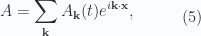
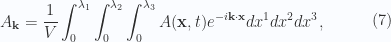
where summation is over all angular wave number triplets . The Fourier coefficients are allowed to be complex valued, as is the resulting four vector , and the associated bivector field .

Fourier inversion, with , follows from

but only this orthogonality relationship and not the Fourier coefficients themselves

will be of interest here. Evaluating the curl for this potential yields

Since the four vector potential has been expressed using an explicit split into time and space components it will be natural to re express the bivector field in terms of scalar and (spatial) vector potentials, with the Fourier coefficients. Writing for the spatial basis vectors, , and , this is

The Faraday bivector field is then

This is now enough to express the energy momentum tensor

It will be more convenient to work with a scalar plus bivector (spatial vector) form of this tensor, and right multiplication by produces such a split

The primary object of this treatment will be consideration of the components of the tensor, which provide a split into energy density , and Poynting vector (momentum density) .

Our first step is to integrate (12) over the volume . This integration and the orthogonality relationship (6), removes the exponentials, leaving

Because commutes with the spatial bivectors, and anticommutes with the spatial vectors, the remainder of the Dirac basis vectors in these expressions can be eliminated

Expanding the energy momentum tensor components.

Energy

In (15) only the bivector-bivector and vector-vector products produce any scalar grades. Except for the bivector product this can be done by inspection. For that part we utilize the identity

This leaves for the energy in the volume

We are left with a completely real expression, and one without any explicit Geometric Algebra. This does not look like the Harmonic oscillator Hamiltonian that was expected. A gauge transformation to eliminate and an observation about when equals zero will give us that, but first lets get the mechanical jobs done, and reduce the products for the field momentum.

Momentum

Now move on to (16). For the factors other than only the vector-bivector products can contribute to the scalar product. We have two such products, one of the form

and the other

The momentum in this volume follows by computation of

All the products are paired in nice conjugates, taking real parts, and premultiplication with gives the desired result. Observe that two of these terms cancel, and another two have no real part. Those last are

Taking the real part of this pure imaginary is zero, leaving just

I am not sure why exactly, but I actually expected a term with , quadratic in the vector potential. Is there a mistake above?

Gauge transformation to simplify the Hamiltonian.

In (20) something that looked like the Harmonic oscillator was expected. On the surface this does not appear to be such a beast. Exploitation of gauge freedom is required to make the simplification that puts things into the Harmonic oscillator form.

If we are to change our four vector potential , then Maxwell’s equation takes the form

which is unchanged by the addition of the gradient to any original potential solution to the equation. In coordinates this is a transformation of the form

and we can use this to force any one of the potential coordinates to zero. For this problem, it appears that it is desirable to seek a such that . That is

Or,

With such a transformation, the and cross term in the Hamiltonian (20) vanishes, as does the term in the four vector square of the last term, leaving just

Additionally, wedging (5) with now does not loose any information so our potential Fourier series is reduced to just

The desired harmonic oscillator form would be had in (26) if it were not for the term. Does that vanish? Returning to Maxwell’s equation should answer that question, but first it has to be expressed in terms of the vector potential. While , the lack of an component means that this can be inverted as

The gradient can also be factored scalar and spatial vector components

So, with this gauge choice the bivector field is

From the left the gradient action on is

and from the right

Taking the difference we have

Which is just

For this vacuum case, premultiplication of Maxwell’s equation by gives

The spatial bivector and trivector grades are all zero. Equating the remaining scalar and vector components to zero separately yields a pair of equations in

If the divergence of the vector potential is constant we have just a wave equation. Let’s see what that divergence is with the assumed Fourier representation

Since , there are two ways for . For each there must be a requirement for either or . The constant solution to the first equation appears to represent a standing spatial wave with no time dependence. Is that of any interest?

The more interesting seeming case is where we have some non-static time varying state. In this case, if , the second of these Maxwell’s equations is just the vector potential wave equation, since the divergence is zero. That is

Solving this isn’t really what is of interest, since the objective was just to determine if the divergence could be assumed to be zero. This shows then, that if the transverse solution to Maxwell’s equation is picked, the Hamiltonian for this field, with this gauge choice, becomes

How does the gauge choice alter the Poynting vector? From (21), all the dependence in that integrated momentum density is lost

The solutions to Maxwell’s equation are seen to result in zero momentum for this infinite periodic field. My expectation was something of the form , so intuition is either failing me, or my math is failing me, or this contrived periodic field solution leads to trouble.

Conclusions and followup.

The objective was met, a reproduction of Bohm’s Harmonic oscillator result using a complex exponential Fourier series instead of separate sine and cosines.

The reason for Bohm’s choice to fix zero divergence as the gauge choice upfront is now clear. That automatically cuts complexity from the results. Figuring out how to work this problem with complex valued potentials and also using the Geometric Algebra formulation probably also made the work a bit more difficult since blundering through both simultaneously was required instead of just one at a time.

This was an interesting exercise though, since doing it this way I am able to understand all the intermediate steps. Bohm employed some subtler argumentation to eliminate the scalar potential upfront, and I have to admit I did not follow his logic, whereas blindly following where the math leads me all makes sense.

As a bit of followup, I’d like to consider the constant case in more detail, and any implications of the freedom to pick .

The general calculation of for the assumed Fourier solution should be possible too, but was not attempted. Doing that general calculation with a four dimensional Fourier series is likely tidier than working with scalar and spatial variables as done here.

Now that the math is out of the way (except possibly for the momentum which doesn’t seem right), some discussion of implications and applications is also in order. My preference is to let the math sink-in a bit first and mull over the momentum issues at leisure.

References

[2] D. Bohm. Quantum Theory. Courier Dover Publications, 1989.

Electrodynamic field energy for vacuum.

[Click here for a PDF of this post with nicer formatting]

Motivation.

We now know how to formulate the energy momentum tensor for complex vector fields (ie. phasors) in the Geometric Algebra formalism. To recap, for the field , where and may be complex vectors we have for Maxwell’s equation

This is a doubly complex representation, with the four vector pseudoscalar acting as a non-commutatitive imaginary, as well as real and imaginary parts for the electric and magnetic field vectors. We take the real part (not the scalar part) of any bivector solution of Maxwell’s equation as the actual solution, but allow ourself the freedom to work with the complex phasor representation when convenient. In these phasor vectors, the imaginary , as in , is a commuting imaginary, commuting with all the multivector elements in the algebra.

The real valued, four vector, energy momentum tensor was found to be

To supply some context that gives meaning to this tensor the associated conservation relationship was found to be

and in particular for , this four vector divergence takes the form

relating the energy term and the Poynting spatial vector with the current density and electric field product that constitutes the energy portion of the Lorentz force density.

Let’s apply this to calculating the energy associated with the field that is periodic within a rectangular prism as done by Bohm in [1]. We do not necessarily need the Geometric Algebra formalism for this calculation, but this will be a fun way to attempt it.

Setup

Let’s assume a Fourier representation for the four vector potential for the field . That is

where summation is over all wave number triplets . The Fourier coefficients are allowed to be complex valued, as is the resulting four vector , and the associated bivector field .

Fourier inversion follows from

but only this orthogonality relationship and not the Fourier coefficients themselves

will be of interest here. Evaluating the curl for this potential yields

We can now form the energy density

With implied summation over all repeated integer indexes (even without matching uppers and lowers), this is

The grade selection used here doesn’t change the result since we already have a scalar, but will just make it convenient to filter out any higher order products that will cancel anyways. Integrating over the volume element and taking advantage of the orthogonality relationship (6), the exponentials are removed, leaving the energy contained in the volume

First reduction of the Hamiltonian.

Let’s take the products involved in sequence one at a time, and evaluate, later adding and taking real parts if required all of

The expectation is to obtain a Hamiltonian for the field that has the structure of harmonic oscillators, where the middle two products would have to be zero or sum to zero or have real parts that sum to zero. The first is expected to contain only products of , and the last only products of .

While initially guessing that (13) and (14) may cancel, this isn’t so obviously the case. The use of cyclic permutation of multivectors within the scalar grade selection operator plus a change of dummy summation indexes in one of the two shows that this sum is of the form . This sum is intrinsically real, so we can neglect one of the two doubling the other, but we will still be required to show that the real part of either is zero.

Lets reduce these one at a time starting with (12), and write temporarily

So the first of our Hamiltonian terms is

Note that summation over is still implied here, so we’d be better off with a spatial vector representation of the Fourier coefficients . With such a notation, this contribution to the Hamiltonian is

To reduce (13) and (13), this time writing , we can start with just the scalar selection

Thus the contribution to the Hamiltonian from (13) and (13) is

Most definitively not zero in general. Our final expansion (15) is the messiest. Again with for short, the grade selection of this term in coordinates is

Expanding this out yields

The contribution to the Hamiltonian from this, with , is then

A final reassembly of the Hamiltonian from the parts (17) and (18) and (21) is then

This is finally reduced to a completely real expression, and one without any explicit Geometric Algebra. All the four vector Fourier vector potentials written out explicitly in terms of the spacetime split , which is natural since an explicit time and space split was the starting point.

Gauge transformation to simplify the Hamiltonian.

While (22) has considerably simpler form than (11), what was expected, was something that looked like the Harmonic oscillator. On the surface this does not appear to be such a beast. Exploitation of gauge freedom is required to make the simplification that puts things into the Harmonic oscillator form.

If we are to change our four vector potential , then Maxwell’s equation takes the form

which is unchanged by the addition of the gradient to any original potential solution to the equation. In coordinates this is a transformation of the form

and we can use this to force any one of the potential coordinates to zero. For this problem, it appears that it is desirable to seek a such that . That is

Or,

With such a transformation, the and cross term in the Hamiltonian (22) vanishes, as does the term in the four vector square of the last term, leaving just

Additionally, wedging (5) with now does not loose any information so our potential Fourier series is reduced to just

The desired harmonic oscillator form would be had in (27) if it were not for the term. Does that vanish? Returning to Maxwell’s equation should answer that question, but first it has to be expressed in terms of the vector potential. While , the lack of an component means that this can be inverted as

The gradient can also be factored scalar and spatial vector components

So, with this gauge choice the bivector field is

From the left the gradient action on is

and from the right

Taking the difference we have

Which is just

For this vacuum case, premultiplication of Maxwell’s equation by gives

The spatial bivector and trivector grades are all zero. Equating the remaining scalar and vector components to zero separately yields a pair of equations in

If the divergence of the vector potential is constant we have just a wave equation. Let’s see what that divergence is with the assumed Fourier representation

Since , there are two ways for . For each there must be a requirement for either or . The constant solution to the first equation appears to represent a standing spatial wave with no time dependence. Is that of any interest?

The more interesting seeming case is where we have some non-static time varying state. In this case, if for all the second of these Maxwell’s equations is just the vector potential wave equation, since the divergence is zero. That is

Solving this isn’t really what is of interest, since the objective was just to determine if the divergence could be assumed to be zero. This shows then, that if the transverse solution to Maxwell’s equation is picked, the Hamiltonian for this field, with this gauge choice, becomes

Conclusions and followup.

The objective was met, a reproduction of Bohm’s Harmonic oscillator result using a complex exponential Fourier series instead of separate sine and cosines.

The reason for Bohm’s choice to fix zero divergence as the gauge choice upfront is now clear. That automatically cuts complexity from the results. Figuring out how to work this problem with complex valued potentials and also using the Geometric Algebra formulation probably also made the work a bit more difficult since blundering through both simultaneously was required instead of just one at a time.

This was an interesting exercise though, since doing it this way I am able to understand all the intermediate steps. Bohm employed some subtler argumentation to eliminate the scalar potential upfront, and I have to admit I did not follow his logic, whereas blindly following where the math leads me all makes sense.

As a bit of followup, I’d like to consider the constant case, and any implications of the freedom to pick . I’d also like to construct the Poynting vector , and see what the structure of that is with this Fourier representation.

A general calculation of for an assumed Fourier solution should be possible too, but working in spatial quantities for the general case is probably torture. A four dimensional Fourier series is likely a superior option for the general case.

References

[1] D. Bohm. Quantum Theory. Courier Dover Publications, 1989.