Peeter Joot's (OLD) Blog.

Math, physics, perl, and programming obscurity.

PHY452H1S Basic Statistical Mechanics. Lecture 18: Fermi gas thermodynamics. Taught by Prof. Arun Paramekanti

Posted by peeterjoot on March 26, 2013

[Click here for a PDF of this post with nicer formatting (especially if my latex to wordpress script has left FORMULA DOES NOT PARSE errors.)]

Disclaimer

Peeter’s lecture notes from class. May not be entirely coherent.

Review

Last time we found that the low temperature behaviour or the chemical potential was quadratic as in fig. 1.1.

\begin{aligned}\mu =\mu(0) - a \frac{T^2}{T_{\mathrm{F}}}\end{aligned} \hspace{\stretch{1}}(1.1.1)

Fig 1.1: Fermi gas chemical potential


Specific heat

\begin{aligned}E = \sum_\mathbf{k} n_{\mathrm{F}}(\epsilon_\mathbf{k}, T) \epsilon_\mathbf{k}\end{aligned} \hspace{\stretch{1}}(1.1.2)

\begin{aligned}\frac{E}{V} &= \frac{1}{{(2\pi)^3}} \int d^3 \mathbf{k} n_{\mathrm{F}}(\epsilon_\mathbf{k}, T) \epsilon_\mathbf{k} \\ &= \int d\epsilon N(\epsilon) n_{\mathrm{F}}(\epsilon, T) \epsilon,\end{aligned} \hspace{\stretch{1}}(1.1.3)

where

\begin{aligned}N(\epsilon) = \frac{1}{{4 \pi^2}}\left( \frac{2m}{\hbar^2} \right)^{3/2}\sqrt{\epsilon}.\end{aligned} \hspace{\stretch{1}}(1.1.4)

Low temperature C_{\mathrm{V}}

\begin{aligned}\frac{\Delta E(T)}{V}=\int_0^\infty d\epsilon N(\epsilon)\left( n_{\mathrm{F}}(\epsilon, T) - n_{\mathrm{F}}(\epsilon, 0) \right)\end{aligned} \hspace{\stretch{1}}(1.1.5)

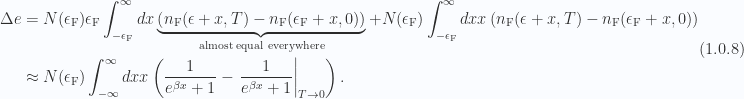
The only change in the distribution fig. 1.2, that is of interest is over the step portion of the distribution, and over this range of interest N(\epsilon) is approximately constant as in fig. 1.3.

Fig 1.2: Fermi distribution

Fig 1.3: Fermi gas density of states
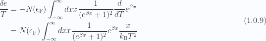
\begin{aligned}N(\epsilon) \approx  N(\mu)\end{aligned} \hspace{\stretch{1}}(1.0.6a)

\begin{aligned}\mu \approx  \epsilon_{\mathrm{F}},\end{aligned} \hspace{\stretch{1}}(1.0.6b)

so that

\begin{aligned}\Delta e \equiv\frac{\Delta E(T)}{V}\approx N(\epsilon_{\mathrm{F}})\int_0^\infty d\epsilon\left( n_{\mathrm{F}}(\epsilon, T) - n_{\mathrm{F}}(\epsilon, 0) \right)=N(\epsilon_{\mathrm{F}})\int_{-\epsilon_{\mathrm{F}}}^\infty d x (\epsilon_{\mathrm{F}} + x)\left( n_{\mathrm{F}}(\epsilon + x, T) - n_{\mathrm{F}}(\epsilon_{\mathrm{F}} + x, 0) \right).\end{aligned} \hspace{\stretch{1}}(1.0.7)

Here we’ve made a change of variables \epsilon = \epsilon_{\mathrm{F}} + x, so that we have near cancelation of the \epsilon_{\mathrm{F}} factor

\begin{aligned}\Delta e &= N(\epsilon_{\mathrm{F}})\epsilon_{\mathrm{F}}\int_{-\epsilon_{\mathrm{F}}}^\infty d x \underbrace{\left( n_{\mathrm{F}}(\epsilon + x, T) - n_{\mathrm{F}}(\epsilon_{\mathrm{F}} + x, 0) \right)}_{\text{almost equal everywhere}}+N(\epsilon_{\mathrm{F}})\int_{-\epsilon_{\mathrm{F}}}^\infty d x x\left( n_{\mathrm{F}}(\epsilon + x, T) - n_{\mathrm{F}}(\epsilon_{\mathrm{F}} + x, 0) \right) \\ &\approx N(\epsilon_{\mathrm{F}})\int_{-\infty}^\infty d x x\left( \frac{1}{{ e^{\beta x} +1 }} - {\left.{{\frac{1}{{ e^{\beta x} +1 }}}}\right\vert}_{{T \rightarrow 0}} \right).\end{aligned} \hspace{\stretch{1}}(1.0.8)

Here we’ve extended the integration range to
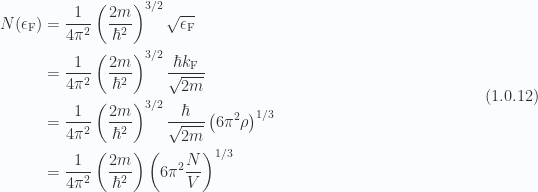
 -\infty since this doesn’t change much. FIXME: justify this to myself? Taking derivatives with respect to temperature we have

\begin{aligned}\frac{\delta e}{T} &= -N(\epsilon_{\mathrm{F}})\int_{-\infty}^\infty d x x\frac{1}{{(e^{\beta x} + 1)^2}}\frac{d}{dT} e^{\beta x} \\ &= N(\epsilon_{\mathrm{F}})\int_{-\infty}^\infty d x x\frac{1}{{(e^{\beta x} + 1)^2}}e^{\beta x}\frac{x}{k_{\mathrm{B}} T^2}\end{aligned} \hspace{\stretch{1}}(1.0.9)

With \beta x = y, we have for T \ll T_{\mathrm{F}}

\begin{aligned}\frac{C}{V} &= N(\epsilon_{\mathrm{F}})\int_{-\infty}^\infty \frac{ dy y^2 e^y }{ (e^y + 1)^2 k_{\mathrm{B}} T^2} (k_{\mathrm{B}} T)^3 \\ &= N(\epsilon_{\mathrm{F}}) k_{\mathrm{B}}^2 T\underbrace{\int_{-\infty}^\infty \frac{ dy y^2 e^y }{ (e^y + 1)^2 } }_{\pi^2/3} \\ &= \frac{\pi^2}{3} N(\epsilon_{\mathrm{F}}) k_{\mathrm{B}} (k_{\mathrm{B}} T).\end{aligned} \hspace{\stretch{1}}(1.0.10)

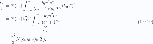
Using eq. 1.1.4 at the Fermi energy and

\begin{aligned}\frac{N}{V} = \rho\end{aligned} \hspace{\stretch{1}}(1.0.11a)

\begin{aligned}\epsilon_{\mathrm{F}} = \frac{\hbar^2 k_{\mathrm{F}}^2}{2 m}\end{aligned} \hspace{\stretch{1}}(1.0.11b)

\begin{aligned}k_{\mathrm{F}} = \left( 6 \pi^2 \rho \right)^{1/3},\end{aligned} \hspace{\stretch{1}}(1.0.11c)

we have

\begin{aligned}N(\epsilon_{\mathrm{F}}) &= \frac{1}{{4 \pi^2}}\left( \frac{2m}{\hbar^2} \right)^{3/2}\sqrt{\epsilon_{\mathrm{F}}} \\ &= \frac{1}{{4 \pi^2}}\left( \frac{2m}{\hbar^2} \right)^{3/2}\frac{\hbar k_{\mathrm{F}}}{\sqrt{2m}} \\ &= \frac{1}{{4 \pi^2}}\left( \frac{2m}{\hbar^2} \right)^{3/2}\frac{\hbar }{\sqrt{2m}} \left( 6 \pi^2 \rho \right)^{1/3} \\ &= \frac{1}{{4 \pi^2}}\left( \frac{2m}{\hbar^2} \right)\left( 6 \pi^2 \frac{N}{V} \right)^{1/3}\end{aligned} \hspace{\stretch{1}}(1.0.12)

Giving

\begin{aligned}\frac{C}{N} &= \frac{\pi^2}{3} \frac{V}{N}\frac{1}{{4 \pi^2}}\left( \frac{2m}{\hbar^2} \right)\left( 6 \pi^2 \frac{N}{V} \right)^{1/3}k_{\mathrm{B}} (k_{\mathrm{B}} T) \\ &= \left( \frac{m}{6 \hbar^2} \right)\left( \frac{V}{N} \right)^{2/3}\left( 6 \pi^2 \right)^{1/3}k_{\mathrm{B}} (k_{\mathrm{B}} T) \\ &= \left( \frac{ \pi^2 m}{3 \hbar^2} \right)\left( \frac{V}{\pi^2 N} \right)^{2/3}k_{\mathrm{B}} (k_{\mathrm{B}} T) \\ &= \left( \frac{ \pi^2 m}{\hbar^2} \right)\frac{\hbar^2}{2 m \epsilon_{\mathrm{F}}}k_{\mathrm{B}} (k_{\mathrm{B}} T),\end{aligned} \hspace{\stretch{1}}(1.0.13)

or

\begin{aligned}\boxed{\frac{C}{N} = \frac{\pi^2}{2} k_{\mathrm{B}} \frac{ k_{\mathrm{B}} T}{\epsilon_{\mathrm{F}}}.}\end{aligned} \hspace{\stretch{1}}(1.0.14)

This is illustrated in fig. 1.4.

Fig 1.4: Specific heat per Fermion


Relativisitic gas

  1. Relativisitic gas

    \begin{aligned}\epsilon_\mathbf{k} = \pm \hbar v \left\lvert {\mathbf{k}} \right\rvert.\end{aligned} \hspace{\stretch{1}}(1.0.15)

    \begin{aligned}\epsilon = \sqrt{(m_0 c^2)^2 + c^2 (\hbar \mathbf{k})^2}\end{aligned} \hspace{\stretch{1}}(1.0.16)

  2. graphene
  3. massless Dirac Fermion

    Fig 1.5: Relativisitic gas energy distribution


    We can think of this state distribution in a condensed matter view, where we can have a hole to electron state transition by supplying energy to the system (i.e. shining light on the substrate). This can also be thought of in a relativisitic particle view where the same state transition can be thought of as a positron electron pair transition. A round trip transition will have to supply energy like 2 m_0 c^2 as illustrated in fig. 1.6.

    Fig 1.6: Hole to electron round trip transition energy requirement


Graphene

Consider graphene, a 2D system. We want to determine the density of states N(\epsilon),

\begin{aligned}\int \frac{d^2 \mathbf{k}}{(2 \pi)^2} \rightarrow \int_{-\infty}^\infty d\epsilon N(\epsilon),\end{aligned} \hspace{\stretch{1}}(1.0.17)

We’ll find a density of states distribution like fig. 1.7.

Fig 1.7: Density of states for 2D linear energy momentum distribution


\begin{aligned}N(\epsilon) = \text{constant factor} \frac{\left\lvert {\epsilon} \right\rvert}{v},\end{aligned} \hspace{\stretch{1}}(1.0.18)

\begin{aligned}C \sim \frac{d}{dT} \int N(\epsilon) n_{\mathrm{F}}(\epsilon) \epsilon d\epsilon,\end{aligned} \hspace{\stretch{1}}(1.0.19)

\begin{aligned}\Delta E \sim \underbrace{T}_{\text{window}}\times\underbrace{T}_{\text{energy}}\times\underbrace{T}_{\text{number of states}}\sim T^3\end{aligned} \hspace{\stretch{1}}(1.0.20)

so that

\begin{aligned}C_{\mathrm{Dimensionless}} \sim T^2\end{aligned} \hspace{\stretch{1}}(1.0.21)

Leave a comment