Peeter Joot's (OLD) Blog.

Math, physics, perl, and programming obscurity.

Bivector form of quantum angular momentum operator (squaring the bivector angular momentum operator)

Posted by peeterjoot on August 28, 2009

[Click here for a PDF of this sequence of posts with nicer formatting]

It is expected that we have the equivalence of the squared bivector form of angular momentum with the classical scalar form in terms of spherical angles \phi, and \theta. Specifically, if no math errors have been made playing around with this GA representation, we should have the following identity for the scalar part of the squared angular momentum operator

\begin{aligned}-\left\langle{{ (\mathbf{x} \wedge \boldsymbol{\nabla})^2 }}\right\rangle =\frac{1}{{\sin\theta}} \frac{\partial {}}{\partial {\theta}} \sin\theta \frac{\partial {}}{\partial {\theta}} + \frac{1}{{\sin^2\theta}} \frac{\partial^2}{\partial \phi^2} \end{aligned} \quad\quad\quad(40)

To finally attempt to verify this we write the angular momentum operator in polar form, using i = \mathbf{e}_1 \mathbf{e}_2 as

\begin{aligned}\mathbf{x} \wedge \boldsymbol{\nabla} &=\hat{\mathbf{r}} \left( \hat{\boldsymbol{\theta}} \partial_\theta + \hat{\boldsymbol{\phi}} \frac{1}{{\sin\theta}} \partial_\phi \right)  \\  \end{aligned}

Expressing the unit vectors in terms of \hat{\boldsymbol{\phi}} and after some rearranging we have

\begin{aligned}\mathbf{x} \wedge \boldsymbol{\nabla} &=I \hat{\boldsymbol{\phi}} \left( \partial_\theta + i e^{I\hat{\boldsymbol{\phi}} \theta} \frac{1}{{\sin\theta}} \partial_\phi \right) \end{aligned} \quad\quad\quad(41)

Using this lets now compute the partials. First for the
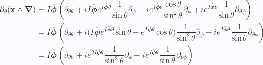
 \theta partials we have

\begin{aligned}\partial_\theta (\mathbf{x} \wedge \boldsymbol{\nabla})&=I \hat{\boldsymbol{\phi}} \left( \partial_{\theta\theta} + i I \hat{\boldsymbol{\phi}} e^{I\hat{\boldsymbol{\phi}} \theta} \frac{1}{{\sin\theta}} \partial_\phi + i e^{I\hat{\boldsymbol{\phi}} \theta} \frac{\cos\theta}{\sin^2\theta} \partial_\phi + i e^{I\hat{\boldsymbol{\phi}} \theta} \frac{1}{{\sin\theta}} \partial_{\theta\phi}\right) \\ &=I \hat{\boldsymbol{\phi}} \left( \partial_{\theta\theta} + i ( I \hat{\boldsymbol{\phi}} e^{I\hat{\boldsymbol{\phi}} \theta} \sin\theta +  e^{I\hat{\boldsymbol{\phi}} \theta} \cos\theta ) \frac{1}{{\sin^2\theta}} \partial_\phi + i e^{I\hat{\boldsymbol{\phi}} \theta} \frac{1}{{\sin\theta}} \partial_{\theta\phi}\right) \\ &=I \hat{\boldsymbol{\phi}} \left( \partial_{\theta\theta} + i e^{2 I\hat{\boldsymbol{\phi}} \theta} \frac{1}{{\sin^2\theta}} \partial_\phi + i e^{I\hat{\boldsymbol{\phi}} \theta} \frac{1}{{\sin\theta}} \partial_{\theta\phi}\right) \\  \end{aligned}

Premultiplying by I\hat{\boldsymbol{\phi}} and taking scalar parts we have the first part of the application of (41) on itself,

\begin{aligned}\left\langle{{ I \hat{\boldsymbol{\phi}} \partial_\theta (\mathbf{x} \wedge \boldsymbol{\nabla}) }}\right\rangle = -\partial_{\theta\theta}  \end{aligned} \quad\quad\quad(42)

For the \phi partials it looks like the simplest option is using the computed bivector \phi partials \partial_\phi (\hat{\mathbf{r}} \hat{\boldsymbol{\theta}}) = \mathbf{e}_3 \hat{\boldsymbol{\phi}}, \partial_\phi (\hat{\mathbf{r}} \hat{\boldsymbol{\phi}}) = -I \hat{\boldsymbol{\phi}} \cos\theta. Doing so we have

\begin{aligned}\partial_\phi (\mathbf{x} \wedge \boldsymbol{\nabla})&=\partial_\phi \left( \hat{\mathbf{r}} \hat{\boldsymbol{\theta}} \partial_\theta + \hat{\mathbf{r}} \hat{\boldsymbol{\phi}} \frac{1}{{\sin\theta}} \partial_\phi \right)  \\ &=\mathbf{e}_3 \hat{\boldsymbol{\phi}} \partial_\theta + +\hat{\mathbf{r}} \hat{\boldsymbol{\theta}} \partial_{\phi\theta} -I \hat{\boldsymbol{\phi}} \cot\theta \partial_\phi + \hat{\mathbf{r}} \hat{\boldsymbol{\phi}} \frac{1}{{\sin\theta}} \partial_{\phi\phi} \end{aligned}

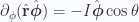
So the remaining terms of the squared angular momentum operator follow by premultiplying by \hat{\mathbf{r}} \hat{\boldsymbol{\phi}}/\sin\theta, and taking scalar parts. This is

\begin{aligned}\left\langle{{ \hat{\mathbf{r}}\hat{\boldsymbol{\phi}} \frac{1}{{\sin\theta}} \partial_\phi (\mathbf{x} \wedge \boldsymbol{\nabla}) }}\right\rangle&=\frac{1}{{\sin\theta}} \left\langle{{-\hat{\mathbf{r}} \mathbf{e}_3 \partial_\theta + -\hat{\boldsymbol{\phi}} \hat{\boldsymbol{\theta}} \partial_{\phi\theta} -\hat{\mathbf{r}} I \cot\theta \partial_\phi }}\right\rangle- \frac{1}{{\sin^2\theta}} \partial_{\phi\phi} \end{aligned}

The second and third terms in the scalar selection have only bivector parts, but since \hat{\mathbf{r}} = \mathbf{e}_3 \cos\theta + \mathbf{e}_1 \sin\theta e^{\mathbf{e}_{12}\phi} has component in the \mathbf{e}_3 direction, we have

\begin{aligned}\left\langle{{ \hat{\mathbf{r}}\hat{\boldsymbol{\phi}} \frac{1}{{\sin\theta}} \partial_\phi (\mathbf{x} \wedge \boldsymbol{\nabla}) }}\right\rangle=-\cot\theta \partial_\theta - \frac{1}{{\sin^2\theta}} \partial_{\phi\phi} \end{aligned} \quad\quad\quad(43)

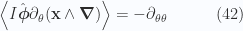
Adding results from (42), and (43) we have

\begin{aligned}-\left\langle{{ (\mathbf{x} \wedge \boldsymbol{\nabla})^2 }}\right\rangle=\partial_{\theta\theta} +\cot\theta \partial_\theta + \frac{1}{{\sin^2\theta}} \partial_{\phi\phi} \end{aligned} \quad\quad\quad(44)

A final verification of (40) now only requires a simple calculus expansion

\begin{aligned}\frac{1}{{\sin\theta}} \frac{\partial {}}{\partial {\theta}} \sin\theta \frac{\partial {}}{\partial {\theta}} \psi&=\frac{1}{{\sin\theta}} \frac{\partial {}}{\partial {\theta}} \sin\theta \partial_\theta \psi \\ &=\frac{1}{{\sin\theta}} (\cos\theta \partial_\theta \psi + \sin\theta \partial_{\theta\theta} \psi) \\ &=\cot\theta \partial_\theta \psi + \partial_{\theta\theta} \psi \end{aligned}

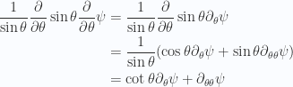
Voila. This exercise demonstrating that what was known to have to be true, is in fact explicitly true, is now done. There’s no new or interesting results in this in and of itself, but we get some additional confidence in the new methods being experimented with.

Leave a comment