April 2024
M	T	W	T	F	S	S
1	2	3	4	5	6	7
8	9	10	11	12	13	14
15	16	17	18	19	20	21
22	23	24	25	26	27	28
29	30

Posts Tagged ‘phy487h1f’

Quadratic Debye

Posted by peeterjoot on January 19, 2014

[Click here for a PDF of this post with nicer formatting]

Question: Quadratic Debye phonons (2013 midterm pr B2)

Assume a quadratic dispersion relation for the longitudinal and transverse modes

$\begin{aligned}\omega = \left\{\begin{array}{l}b_{\mathrm{L}} q^2 \\ b_{\mathrm{T}} q^2\end{array}\right..\end{aligned} \hspace{\stretch{1}}(1.2)$

Part a

Find the density of states.

Part b

Find the Debye frequency.

Part c

In terms of $k_{\mathrm{B}} \Theta = \hbar \omega_{\mathrm{D}}$ , and

$\begin{aligned}\mathcal{I} = \int_0^\infty \frac{y^{5/2} e^{y} dy}{\left( { e^y - 1} \right)^2 },\end{aligned} \hspace{\stretch{1}}(1.2)$

find the specific heat for $k_{\mathrm{B}} T \ll \hbar \omega_{\mathrm{D}}$ .

Part d

Find the specific heat for $k_{\mathrm{B}} T \gg \hbar \omega_{\mathrm{D}}$ .

Answer

Part a

Working straight from the definition

$\begin{aligned}Z(\omega) &= \frac{V}{(2 \pi)^3 } \sum_{L, T} \int \frac{df_\omega}{ \left\lvert { \boldsymbol{\nabla}_\mathbf{q} \omega } \right\rvert } \\ &= \frac{V}{(2 \pi)^3 } \left( { {\left.{{\frac{4 \pi q^2}{2 b_{\mathrm{L}} q} }}\right\vert}_{{\mathrm{L}}} + {\left.{{\frac{2 \times 4 \pi q^2}{2 b_{\mathrm{T}} q} }}\right\vert}_{{\mathrm{T}}} } \right) \\ &= \frac{V}{4 \pi^2 } \left( { \frac{q_{\mathrm{L}}}{b_{\mathrm{L}}} + \frac{2 q_{\mathrm{T}}}{b_{\mathrm{T}}} } \right).\end{aligned} \hspace{\stretch{1}}(1.3)$

With $q_{\mathrm{L}} = \sqrt{\omega/b_{\mathrm{L}}}$ and $q_{\mathrm{T}} = \sqrt{\omega/b_{\mathrm{T}}}$ , this is

$\begin{aligned}Z(\omega) = \frac{V}{4 \pi^2 } \left( { \frac{1}{b_{\mathrm{L}}^{3/2}} + \frac{2}{b_{\mathrm{T}}^{3/2}} } \right)\sqrt{\omega}\end{aligned} \hspace{\stretch{1}}(1.4)$

Part b

The Debye frequency was given implicitly by

$\begin{aligned}\int_0^{\omega_{\mathrm{D}}} Z(\omega) d\omega = 3 r N,\end{aligned} \hspace{\stretch{1}}(1.5)$

which gives

$\begin{aligned}3 r N=\frac{2}{3} \frac{V}{4 \pi^2 } \left( { \frac{1}{b_{\mathrm{L}}^{3/2}} + \frac{2}{b_{\mathrm{T}}^{3/2}} } \right)\omega_{\mathrm{D}}^{3/2}=\frac{V}{6 \pi^2 } \left( { \frac{1}{b_{\mathrm{L}}^{3/2}} + \frac{2}{b_{\mathrm{T}}^{3/2}} } \right)\omega_{\mathrm{D}}^{3/2}\end{aligned} \hspace{\stretch{1}}(1.6)$

Part c

Assuming a Bose distribution and ignoring the zero point energy, which has no temperature dependence, the specific heat, the temperature derivative of the energy density, is

$\begin{aligned}C_{\mathrm{V}} &= \frac{d}{d T} \frac{1}{{V}} \int Z(\omega) \frac{\hbar \omega}{ e^{\hbar \omega/ k_{\mathrm{B}} T } - 1} d\omega \\ &= \frac{1}{{V}} \frac{d}{d T} \int Z(\omega) \frac{\hbar \omega}{ \hbar \omega/ k_{\mathrm{B}} T + \frac{1}{{2}}( \hbar \omega/k_{\mathrm{B}} T)^2 + \cdots } d\omega \\ &\approx \frac{1}{{V}} \frac{d}{d T} \int Z(\omega) k_{\mathrm{B}} T d\omega \\ &= \frac{1}{{V}} k_{\mathrm{B}} 3 r N.\end{aligned} \hspace{\stretch{1}}(1.7)$

Part d

First note that the density of states can be written

$\begin{aligned}Z(\omega) = \frac{9 r N}{ 2 \omega_{\mathrm{D}}^{3/2} } \omega^{1/2},\end{aligned} \hspace{\stretch{1}}(1.8)$

for a specific heat of

$\begin{aligned}C_{\mathrm{V}} &= \frac{d}{d T} \frac{1}{{V}} \int_0^\infty \frac{9 r N}{ 2 \omega_{\mathrm{D}}^{3/2} } \omega^{1/2} \frac{\hbar \omega}{ e^{\hbar \omega/ k_{\mathrm{B}} T } - 1} d\omega \\ &= \frac{9 r N}{ 2 V \omega_{\mathrm{D}}^{3/2} } \int_0^\infty d\omega \omega^{1/2} \frac{d}{d T} \frac{\hbar \omega}{ e^{\hbar \omega/ k_{\mathrm{B}} T } - 1} \\ &= \frac{9 r N}{ 2 V \omega_{\mathrm{D}}^{3/2} } \int_0^\infty d\omega \omega^{1/2} \frac{-\hbar \omega}{ \left( {e^{\hbar \omega/ k_{\mathrm{B}} T } - 1} \right)^2 } e^{\hbar \omega/k_{\mathrm{B}} T} \hbar \omega/k_{\mathrm{B}} \left( {-\frac{1}{{T^2}}} \right) \\ &= \frac{9 r N k_{\mathrm{B}} }{ 2 V \omega_{\mathrm{D}}^{3/2} } \left( { \frac{ k_{\mathrm{B}} T}{\hbar} } \right)^{3/2}\int_0^\infty d \frac{\hbar \omega}{k_{\mathrm{B}} T} \left( {\frac{\hbar \omega}{k_{\mathrm{B}} T}} \right)^{1/2} \frac{1}{ \left( {e^{\hbar \omega/ k_{\mathrm{B}} T } - 1} \right)^2 } e^{\hbar \omega/k_{\mathrm{B}} T} \left( { \frac{\hbar \omega}{k_{\mathrm{B}} T} } \right)^2 \\ &= \frac{9 r N k_{\mathrm{B}} }{ 2 V \omega_{\mathrm{D}}^{3/2} } \left( { \frac{ k_{\mathrm{B}} T}{\hbar} } \right)^{3/2}\int_0^\infty dy \frac{y^{5/2} e^y }{ \left( {e^y - 1} \right)^2 } \\& = \frac{9 r N k_{\mathrm{B}} }{ 2 V } \left( { \frac{ T}{\Theta} } \right)^{3/2} \mathcal{I}.\end{aligned} \hspace{\stretch{1}}(1.9)$

Posted in Math and Physics Learning. | Tagged: Condensed matter physics, Debye frequency, Debye temperature, density of states, phonon, phy487h1f | Leave a Comment »

One atom basis phonons in 2D

Posted by peeterjoot on January 19, 2014

[Click here for a PDF of this post with nicer formatting]

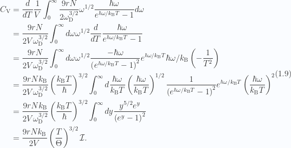
Let’s tackle a problem like the 2D problem of the final exam, but first more generally. Instead of a square lattice consider the lattice with the geometry illustrated in fig. 1.1.

Fig 1.1: Oblique one atom basis

Here, $\mathbf{a}$ and $\mathbf{b}$ are the vector differences between the equilibrium positions separating the masses along the $K_1$ and $K_2$ interaction directions respectively. The equilibrium spacing for the cross coupling harmonic forces are

$\begin{aligned}\begin{aligned}\mathbf{r} &= (\mathbf{b} + \mathbf{a})/2 \\ \mathbf{s} &= (\mathbf{b} - \mathbf{a})/2.\end{aligned}\end{aligned} \hspace{\stretch{1}}(1.1)$

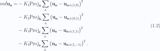
Based on previous calculations, we can write the equations of motion by inspection

$\begin{aligned}\begin{aligned}m \dot{d}{\mathbf{u}}_\mathbf{n} = &-K_1 \text{Proj}_{\hat{\mathbf{a}}} \sum_\pm \left( { \mathbf{u}_\mathbf{n} - \mathbf{u}_{\mathbf{n} \pm(1, 0)}} \right)^2 \\ &-K_2 \text{Proj}_{\hat{\mathbf{b}}} \sum_\pm \left( { \mathbf{u}_\mathbf{n} - \mathbf{u}_{\mathbf{n} \pm(0, 1)}} \right)^2 \\ &-K_3 \text{Proj}_{\hat{\mathbf{r}}} \sum_\pm \left( { \mathbf{u}_\mathbf{n} - \mathbf{u}_{\mathbf{n} \pm(1, 1)}} \right)^2 \\ &-K_4 \text{Proj}_{\hat{\mathbf{s}}} \sum_\pm \left( { \mathbf{u}_\mathbf{n} - \mathbf{u}_{\mathbf{n} \pm(1, -1)}} \right)^2.\end{aligned}\end{aligned} \hspace{\stretch{1}}(1.2)$

Inserting the trial solution

$\begin{aligned}\mathbf{u}_\mathbf{n} = \frac{1}{{\sqrt{m}}} \boldsymbol{\epsilon}(\mathbf{q}) e^{i( \mathbf{r}_\mathbf{n} \cdot \mathbf{q} - \omega t) },\end{aligned} \hspace{\stretch{1}}(1.3)$

and using the matrix form for the projection operators, we have

$\begin{aligned}\begin{aligned}\omega^2 \boldsymbol{\epsilon} &=\frac{K_1}{m} \hat{\mathbf{a}} \hat{\mathbf{a}}^\text{T} \boldsymbol{\epsilon}\sum_\pm\left( { 1 - e^{\pm i \mathbf{a} \cdot \mathbf{q}} } \right) \\ & +\frac{K_2}{m} \hat{\mathbf{b}} \hat{\mathbf{b}}^\text{T} \boldsymbol{\epsilon}\sum_\pm\left( { 1 - e^{\pm i \mathbf{b} \cdot \mathbf{q}} } \right) \\ & +\frac{K_3}{m} \hat{\mathbf{b}} \hat{\mathbf{b}}^\text{T} \boldsymbol{\epsilon}\sum_\pm\left( { 1 - e^{\pm i (\mathbf{b} + \mathbf{a}) \cdot \mathbf{q}} } \right) \\ & +\frac{K_3}{m} \hat{\mathbf{b}} \hat{\mathbf{b}}^\text{T} \boldsymbol{\epsilon}\sum_\pm\left( { 1 - e^{\pm i (\mathbf{b} - \mathbf{a}) \cdot \mathbf{q}} } \right) \\ &=\frac{4 K_1}{m} \hat{\mathbf{a}} \hat{\mathbf{a}}^\text{T} \boldsymbol{\epsilon} \sin^2\left( { \mathbf{a} \cdot \mathbf{q}/2 } \right)+\frac{4 K_2}{m} \hat{\mathbf{b}} \hat{\mathbf{b}}^\text{T} \boldsymbol{\epsilon} \sin^2\left( { \mathbf{b} \cdot \mathbf{q}/2 } \right) \\ &+\frac{4 K_3}{m} \hat{\mathbf{r}} \hat{\mathbf{r}}^\text{T} \boldsymbol{\epsilon} \sin^2\left( { (\mathbf{b} + \mathbf{a}) \cdot \mathbf{q}/2 } \right)+\frac{4 K_4}{m} \hat{\mathbf{s}} \hat{\mathbf{s}}^\text{T} \boldsymbol{\epsilon} \sin^2\left( { (\mathbf{b} - \mathbf{a}) \cdot \mathbf{q}/2 } \right).\end{aligned}\end{aligned} \hspace{\stretch{1}}(1.4)$

This fully specifies our eigenvalue problem. Writing

$\begin{aligned}\begin{aligned}S_1 &= \sin^2\left( { \mathbf{a} \cdot \mathbf{q}/2 } \right) \\ S_2 &= \sin^2\left( { \mathbf{b} \cdot \mathbf{q}/2 } \right) \\ S_3 &= \sin^2\left( { (\mathbf{b} + \mathbf{a}) \cdot \mathbf{q}/2 } \right) \\ S_4 &= \sin^2\left( { (\mathbf{b} - \mathbf{a}) \cdot \mathbf{q}/2 } \right)\end{aligned}\end{aligned} \hspace{\stretch{1}}(1.0.5.5)$

$\begin{aligned}\boxed{A = \frac{4}{m}\left( { K_1 S_1 \hat{\mathbf{a}} \hat{\mathbf{a}}^\text{T} + K_2 S_2 \hat{\mathbf{b}} \hat{\mathbf{b}}^\text{T} + K_3 S_3 \hat{\mathbf{r}} \hat{\mathbf{r}}^\text{T} + K_4 S_4 \hat{\mathbf{s}} \hat{\mathbf{s}}^\text{T}} \right),}\end{aligned} \hspace{\stretch{1}}(1.0.5.5)$

we wish to solve

$\begin{aligned}A \boldsymbol{\epsilon} = \omega^2 \boldsymbol{\epsilon} = \lambda \boldsymbol{\epsilon}.\end{aligned} \hspace{\stretch{1}}(1.0.6)$

Neglecting the specifics of the matrix at hand, consider a generic two by two matrix

$\begin{aligned}A = \begin{bmatrix}a & b \\ c & d\end{bmatrix},\end{aligned} \hspace{\stretch{1}}(1.0.6)$

for which the characteristic equation is

$\begin{aligned}0 &= \begin{vmatrix}\lambda - a & - b \\ -c & \lambda -d \end{vmatrix} \\ &= (\lambda - a)(\lambda - d) - b c \\ &= \lambda^2 - (a + d) \lambda + a d - b c \\ &= \lambda^2 - (Tr A) \lambda + \left\lvert {A} \right\rvert \\ &= \left( {\lambda - \frac{Tr A}{2}} \right)^2- \left( {\frac{Tr A}{2}} \right)^2 + \left\lvert {A} \right\rvert.\end{aligned} \hspace{\stretch{1}}(1.0.6)$

So our angular frequencies are given by

$\begin{aligned}\omega^2 = \frac{1}{{2}} \left( { Tr A \pm \sqrt{ \left(Tr A\right)^2 - 4 \left\lvert {A} \right\rvert }} \right).\end{aligned} \hspace{\stretch{1}}(1.0.6)$

The square root can be simplified slightly

$\begin{aligned}\left( {Tr A} \right)^2 - 4 \left\lvert {A} \right\rvert \\ &= (a + d)^2 -4 (a d - b c) \\ &= a^2 + d^2 + 2 a d - 4 a d + 4 b c \\ &= (a - d)^2 + 4 b c,\end{aligned} \hspace{\stretch{1}}(1.0.6)$

so that, finally, the dispersion relation is

$\begin{aligned}\boxed{\omega^2 = \frac{1}{{2}} \left( { d + a \pm \sqrt{ (d - a)^2 + 4 b c } } \right),}\end{aligned} \hspace{\stretch{1}}(1.0.6)$

Our eigenvectors will be given by

$\begin{aligned}0 = (\lambda - a) \boldsymbol{\epsilon}_1 - b\boldsymbol{\epsilon}_2,\end{aligned} \hspace{\stretch{1}}(1.0.6)$

$\begin{aligned}\boldsymbol{\epsilon}_1 \propto \frac{b}{\lambda - a}\boldsymbol{\epsilon}_2.\end{aligned} \hspace{\stretch{1}}(1.0.6)$

So, our eigenvectors, the vectoral components of our atomic displacements, are

$\begin{aligned}\boldsymbol{\epsilon} \propto\begin{bmatrix}b \\ \omega^2 - a\end{bmatrix},\end{aligned} \hspace{\stretch{1}}(1.0.6)$

$\begin{aligned}\boxed{\boldsymbol{\epsilon} \propto\begin{bmatrix}2 b \\ d - a \pm \sqrt{ (d - a)^2 + 4 b c }\end{bmatrix}.}\end{aligned} \hspace{\stretch{1}}(1.0.6)$

Square lattice

There is not too much to gain by expanding out the projection operators explicitly in general. However, let’s do this for the specific case of a square lattice (as on the exam problem). In that case, our projection operators are

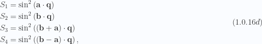
$\begin{aligned}\hat{\mathbf{a}} \hat{\mathbf{a}}^\text{T} = \begin{bmatrix}1 \\ 0\end{bmatrix}\begin{bmatrix}1 & 0\end{bmatrix}=\begin{bmatrix}1 & 0 \\ 0 & 0\end{bmatrix}\end{aligned} \hspace{\stretch{1}}(1.0.16a)$

$\begin{aligned}\hat{\mathbf{b}} \hat{\mathbf{b}}^\text{T} = \begin{bmatrix}0\\ 1 \end{bmatrix}\begin{bmatrix}0 &1 \end{bmatrix}=\begin{bmatrix}0 & 0 \\ 0 & 1\end{bmatrix}\end{aligned} \hspace{\stretch{1}}(1.0.16b)$

$\begin{aligned}\hat{\mathbf{r}} \hat{\mathbf{r}}^\text{T} = \frac{1}{{2}}\begin{bmatrix}1 \\ 1 \end{bmatrix}\begin{bmatrix}1 &1 \end{bmatrix}=\frac{1}{{2}}\begin{bmatrix}1 & 1 \\ 1 & 1\end{bmatrix}\end{aligned} \hspace{\stretch{1}}(1.0.16c)$

$\begin{aligned}\hat{\mathbf{s}} \hat{\mathbf{s}}^\text{T} = \frac{1}{{2}}\begin{bmatrix}-1 \\ 1 \end{bmatrix}\begin{bmatrix}-1 &1 \end{bmatrix}=\frac{1}{{2}}\begin{bmatrix}1 & -1 \\ -1 & 1\end{bmatrix}\end{aligned} \hspace{\stretch{1}}(1.0.16d)$

$\begin{aligned}\begin{aligned}S_1 &= \sin^2\left( { \mathbf{a} \cdot \mathbf{q} } \right) \\ S_2 &= \sin^2\left( { \mathbf{b} \cdot \mathbf{q} } \right) \\ S_3 &= \sin^2\left( { (\mathbf{b} + \mathbf{a}) \cdot \mathbf{q} } \right) \\ S_4 &= \sin^2\left( { (\mathbf{b} - \mathbf{a}) \cdot \mathbf{q} } \right),\end{aligned}\end{aligned} \hspace{\stretch{1}}(1.0.16d)$

Our matrix is

$\begin{aligned}A = \frac{2}{m}\begin{bmatrix}2 K_1 S_1 + K_3 S_3 + K_4 S_4 & K_3 S_3 - K_4 S_4 \\ K_3 S_3 - K_4 S_4 & 2 K_2 S_2 + K_3 S_3 + K_4 S_4\end{bmatrix},\end{aligned} \hspace{\stretch{1}}(1.0.16d)$

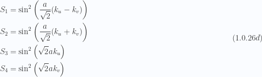
where, specifically, the squared sines for this geometry are

$\begin{aligned}S_1 = \sin^2 \left( { \mathbf{a} \cdot \mathbf{q}/2 } \right) = \sin^2 \left( { a q_x/2} \right)\end{aligned} \hspace{\stretch{1}}(1.0.19a)$

$\begin{aligned}S_2 = \sin^2 \left( { \mathbf{b} \cdot \mathbf{q}/2 } \right) = \sin^2 \left( { a q_y/2} \right)\end{aligned} \hspace{\stretch{1}}(1.0.19b)$

$\begin{aligned}S_3 = \sin^2 \left( { (\mathbf{b} + \mathbf{a}) \cdot \mathbf{q}/2 } \right) = \sin^2 \left( { a (q_x + q_y)/2} \right)\end{aligned} \hspace{\stretch{1}}(1.0.19c)$

$\begin{aligned}S_4 = \sin^2 \left( { (\mathbf{b} - \mathbf{a}) \cdot \mathbf{q}/2 } \right) = \sin^2 \left( { a (q_y - q_x)/2} \right).\end{aligned} \hspace{\stretch{1}}(1.0.19d)$

Using eq. 1.0.6, the dispersion relation and eigenvectors are

$\begin{aligned}\omega^2 = \frac{2}{m} \left( { \sum_i K_i S_i \pm \sqrt{ (K_2 S_2 - K_1 S_1)^2 + (K_3 S_3 - K_4 S_4)^2 } } \right)\end{aligned} \hspace{\stretch{1}}(1.0.20.20)$

$\begin{aligned}\boldsymbol{\epsilon} \propto\begin{bmatrix}K_3 S_3 - K_4 S_4 \\ K_2 S_2 - K_1 S_1 \pm \sqrt{ (K_2 S_2 - K_1 S_1)^2 + (K_3 S_3 - K_4 S_4)^2 } \end{bmatrix}.\end{aligned} \hspace{\stretch{1}}(1.0.20.20)$

This calculation is confirmed in oneAtomBasisPhononSquareLatticeEigensystem.nb. Mathematica calculates an alternate form (equivalent to using a zero dot product for the second row), of

$\begin{aligned}\boldsymbol{\epsilon} \propto\begin{bmatrix}K_1 S_1 - K_2 S_2 \pm \sqrt{ (K_2 S_2 - K_1 S_1)^2 + (K_3 S_3 - K_4 S_4)^2 } \\ K_3 S_3 - K_4 S_4 \end{bmatrix}.\end{aligned} \hspace{\stretch{1}}(1.0.20.20)$

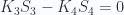
Either way, we see that $K_3 S_3 - K_4 S_4 = 0$ leads to only horizontal or vertical motion.

With the exam criteria

In the specific case that we had on the exam where $K_1 = K_2$ and $K_3 = K_4$ , these are

$\begin{aligned}\omega^2 = \frac{2}{m} \left( { K_1 (S_1 + S_2) + K_3(S_3 + S_4) \pm \sqrt{ K_1^2 (S_2 - S_1)^2 + K_3^2 (S_3 - S_4)^2 } } \right)\end{aligned} \hspace{\stretch{1}}(1.0.22.22)$

$\begin{aligned}\boldsymbol{\epsilon} \propto\begin{bmatrix}K_3 \left( { S_3 - S_4 } \right) \\ K_1 \left( { (S_1 - S_2) \pm \sqrt{ (S_2 - S_1)^2 + \left( \frac{K_3}{K_1} \right)^2 (S_3 - S_4)^2 } } \right)\end{bmatrix}.\end{aligned} \hspace{\stretch{1}}(1.0.22.22)$

For horizontal and vertical motion we need $S_3 = S_4$ , or for a $2 \pi \times \text{integer}$ difference in the absolute values of the sine arguments

$\begin{aligned}\pm ( a (q_x + q_y) /2 ) = a (q_y - q_y) /2 + 2 \pi n.\end{aligned} \hspace{\stretch{1}}(1.0.22.22)$

That is, one of

$\begin{aligned}\begin{aligned}q_x &= \frac{2 \pi}{a} n \\ q_y &= \frac{2 \pi}{a} n\end{aligned}\end{aligned} \hspace{\stretch{1}}(1.0.22.22)$

In the first BZ, that is one of $q_x = 0$ or $q_y = 0$ .

System in rotated coordinates

On the exam, where we were asked to solve for motion along the cross directions explicitly, there was a strong hint to consider a rotated (by $\pi/4$ ) coordinate system.

The rotated the lattice basis vectors are $\mathbf{a} = a \mathbf{e}_1, \mathbf{b} = a \mathbf{e}_2$ , and the projection matrices. Writing $\hat{\mathbf{r}} = \mathbf{f}_1$ and $\hat{\mathbf{s}} = \mathbf{f}_2$ , where $\mathbf{f}_1 = (\mathbf{e}_1 + \mathbf{e}_2)/\sqrt{2}, \mathbf{f}_2 = (\mathbf{e}_2 - \mathbf{e}_1)/\sqrt{2}$ , or $\mathbf{e}_1 = (\mathbf{f}_1 - \mathbf{f}_2)/\sqrt{2}, \mathbf{e}_2 = (\mathbf{f}_1 + \mathbf{f}_2)/\sqrt{2}$ . In the $\{\mathbf{f}_1, \mathbf{f}_2\}$ basis the projection matrices are

$\begin{aligned}\hat{\mathbf{a}} \hat{\mathbf{a}}^\text{T} = \frac{1}{{2}}\begin{bmatrix}1 \\ -1\end{bmatrix}\begin{bmatrix}1 & -1\end{bmatrix}= \frac{1}{{2}} \begin{bmatrix}1 & -1 \\ -1 & 1\end{bmatrix}\end{aligned} \hspace{\stretch{1}}(1.0.25a)$

$\begin{aligned}\hat{\mathbf{b}} \hat{\mathbf{b}}^\text{T} = \frac{1}{{2}}\begin{bmatrix}1 \\ 1\end{bmatrix}\begin{bmatrix}1 & 1\end{bmatrix}= \frac{1}{{2}} \begin{bmatrix}1 & 1 \\ 1 & 1\end{bmatrix}\end{aligned} \hspace{\stretch{1}}(1.0.25b)$

$\begin{aligned}\hat{\mathbf{r}} \hat{\mathbf{r}}^\text{T} = \begin{bmatrix}1 & 0 \\ 0 & 0\end{bmatrix}\end{aligned} \hspace{\stretch{1}}(1.0.25c)$

$\begin{aligned}\hat{\mathbf{s}} \hat{\mathbf{s}}^\text{T} = \begin{bmatrix}0 & 0 \\ 0 & 1\end{bmatrix}\end{aligned} \hspace{\stretch{1}}(1.0.25d)$

The dot products that show up in the squared sines are

$\begin{aligned}\mathbf{a} \cdot \mathbf{q}=a \frac{1}{{\sqrt{2}}} (\mathbf{f}_1 - \mathbf{f}_2) \cdot (\mathbf{f}_1 k_u + \mathbf{f}_2 k_v)=\frac{a}{\sqrt{2}} (k_u - k_v)\end{aligned} \hspace{\stretch{1}}(1.0.26a)$

$\begin{aligned}\mathbf{b} \cdot \mathbf{q}=a \frac{1}{{\sqrt{2}}} (\mathbf{f}_1 + \mathbf{f}_2) \cdot (\mathbf{f}_1 k_u + \mathbf{f}_2 k_v)=\frac{a}{\sqrt{2}} (k_u + k_v)\end{aligned} \hspace{\stretch{1}}(1.0.26b)$

$\begin{aligned}(\mathbf{a} + \mathbf{b}) \cdot \mathbf{q} = \sqrt{2} a k_u \end{aligned} \hspace{\stretch{1}}(1.0.26c)$

$\begin{aligned}(\mathbf{b} - \mathbf{a}) \cdot \mathbf{q} = \sqrt{2} a k_v \end{aligned} \hspace{\stretch{1}}(1.0.26d)$

So that in this basis

$\begin{aligned}\begin{aligned}S_1 &= \sin^2 \left( { \frac{a}{\sqrt{2}} (k_u - k_v) } \right) \\ S_2 &= \sin^2 \left( { \frac{a}{\sqrt{2}} (k_u + k_v) } \right) \\ S_3 &= \sin^2 \left( { \sqrt{2} a k_u } \right) \\ S_4 &= \sin^2 \left( { \sqrt{2} a k_v } \right)\end{aligned}\end{aligned} \hspace{\stretch{1}}(1.0.26d)$

With the rotated projection operators eq. 1.0.5.5 takes the form

$\begin{aligned}A = \frac{2}{m}\begin{bmatrix}K_1 S_1 + K_2 S_2 + 2 K_3 S_3 & K_2 S_2 - K_1 S_1 \\ K_2 S_2 - K_1 S_1 & K_1 S_1 + K_2 S_2 + 2 K_4 S_4\end{bmatrix}.\end{aligned} \hspace{\stretch{1}}(1.0.26d)$

This clearly differs from eq. 1.0.16d, and results in a different expression for the eigenvectors, but the same as eq. 1.0.20.20 for the angular frequencies.

$\begin{aligned}\boldsymbol{\epsilon} \propto\begin{bmatrix}K_2 S_2 - K_1 S_1 \\ K_4 S_4 - K_3 S_3 \mp \sqrt{ (K_2 S_2 - K_1 S_1)^2 + (K_3 S_3 - K_4 S_4)^2 }\end{bmatrix},\end{aligned} \hspace{\stretch{1}}(1.0.26d)$

or, equivalently

$\begin{aligned}\boldsymbol{\epsilon} \propto\begin{bmatrix}K_4 S_4 - K_3 S_3 \mp \sqrt{ (K_2 S_2 - K_1 S_1)^2 + (K_3 S_3 - K_4 S_4)^2 } \\ K_1 S_1 - K_2 S_2 \\ \end{bmatrix},\end{aligned} \hspace{\stretch{1}}(1.0.26d)$

For the $K_1 = K_2$ and $K_3 = K_4$ case of the exam, this is

$\begin{aligned}\boldsymbol{\epsilon} \propto\begin{bmatrix}K_1 (S_2 - S_1 ) \\ K_3 \left( { S_4 - S_3 \mp \sqrt{ \left( \frac{K_1}{K_3} \right)^2 (S_2 - S_1)^2 + (S_3 - S_4)^2 } } \right)\end{bmatrix}.\end{aligned} \hspace{\stretch{1}}(1.0.26d)$

Similar to the horizontal coordinate system, we see that we have motion along the diagonals when

$\begin{aligned}\pm \frac{a}{\sqrt{2}} (k_u - k_v) = \frac{a}{\sqrt{2}} (k_u + k_v) + 2 \pi n,\end{aligned} \hspace{\stretch{1}}(1.0.26d)$

or one of

$\begin{aligned}\begin{aligned}k_u &= \sqrt{2} \frac{\pi}{a} n \\ k_v &= \sqrt{2} \frac{\pi}{a} n\end{aligned}\end{aligned} \hspace{\stretch{1}}(1.0.26d)$

Stability?

The exam asked why the cross coupling is required for stability. Clearly we have more complex interaction. The constant $\omega$ surfaces will also be more complex. However, I still don’t have a good intuition what exactly was sought after for that part of the question.

Numerical computations

A Manipulate allowing for choice of the spring constants and lattice orientation, as shown in fig. 1.2, is available in phy487/oneAtomBasisPhonon.nb. This interface also provides a numerical calculation of the distribution relation as shown in fig. 1.3, and provides an animation of the normal modes for any given selection of $\mathbf{q}$ and $\omega(\mathbf{q})$ (not shown).

Fig 1.2: 2D Single atom basis Manipulate interface

Fig 1.3: Sample distribution relation for 2D single atom basis.

Posted in Math and Physics Learning. | Tagged: angular frequency, Condensed matter physics, dispersion relation, harmonic oscillator, one atom basis, phonon, phy487h1f | Leave a Comment »

First post of phy487 (Condensed Matter Physics) notes posted.

Posted by peeterjoot on October 4, 2013

I’ve posted a first (incomplete) draft of my lecture notes for the Winter 2013, University of Toronto Condensed Matter Physics course (PHY487H1F), taught by Prof. Stephen Julian.

Official course description:

“Introduction to the concepts used in the modern treatment of solids. The student is assumed to be familiar with elementary quantum mechanics. Topics include: bonding in solids, crystal structures, lattice vibrations, free electron model of metals, band structure, thermal properties, magnetism and superconductivity (time permitting).”

In this course there will be an attempt to cover

Bonding and crystal structure: Why solids form, describing periodic order mathematically, diffraction.
Lattice vibrations: .elementary excitation. of a periodic array of atoms (periodicity allows a 10 23 body problem to be solved).
Electrons in solids: Explaining this introduces a need for quantum mechanics. Periodicity -> band structure -> insulators vs metals.
Electrical conduction in solids. (metals and semiconductors).

This document contains:

Plain old lecture notes. These mirror what was covered in class, possibly augmented with additional details.
Personal notes exploring details that were not clear to me from the lectures, or from the texts associated with the lecture material.
Assigned problems. Like anything else take these as is. I may or may not have gone back and corrected errors, and did not see the graded versions of the last two problem sets.
Some worked problems attempted as course prep, for fun, or for test preparation, or post test reflection.
Links to Mathematica workbooks associated with these notes.

Posted in Math and Physics Learning. | Tagged: 1 atom basis, alkali metal, atomic scattering factor, BCC, Body centered cubic, Bragg condition, Bravais, conventional unit cell, Diamond lattice, dynamical matrix, elastic scattering, Face centered cubic, FCC, filling factor, HCP, hexagonal close packed, hybridization, Laue condition, Madelung constant, melting point, metallic bond, Miller indices, nn, noble gas, phy487, phy487h1, phy487h1f, promotion, reciprocal vectors, Simple cubic, structure factor, transition metal, Van der Waals, Van Der Walls bonding | 4 Comments »

	Determining the alig… on C structure alignment pad…
	Manas shetty on Cartesian to spherical change…
	peeterjoot on Derivative recurrence relation…
	Daniel Pires on Derivative recurrence relation…
	peeterjoot on Curious problem using the vari…

Peeter Joot's (OLD) Blog.

Math, physics, perl, and programming obscurity.

Categories

Archives

Recent Posts

Meta

Recent Comments

People not reading this blog: 7,179,979,522 minus:

Subscribe

Posts Tagged ‘phy487h1f’

Quadratic Debye

Question: Quadratic Debye phonons (2013 midterm pr B2)

Part a

Part b

Part c

Part d

Answer

Part a

Part b

Part c

Part d

One atom basis phonons in 2D

First post of phy487 (Condensed Matter Physics) notes posted.