Obsolete with potential errors.
This post may be in error. I wrote this before understanding that the gradient used in Stokes Theorem must be projected onto the tangent space of the parameterized surface, as detailed in Alan MacDonald’s Vector and Geometric Calculus.
See the post ‘stokes theorem in geometric algebra‘ [PDF], where this topic has been revisited with this in mind.
Original Post:
[Click here for a PDF of this post with nicer formatting]
Motivation.
I’ve worked through Stokes theorem concepts a couple times on my own now. One of the first times, I was trying to formulate this in a Geometric Algebra context. I had to resort to a tensor decomposition, and pictures, before ending back in the Geometric Algebra description. Later I figured out how to do it entirely with a Geometric Algebra description, and was able to eliminate reliance on the pictures that made the path to generalization to higher dimensional spaces unclear.
It’s my expectation that if one started with a tensor description, the proof entirely in tensor form would not be difficult. This is what I’d like to try this time. To start off, I’ll temporarily use the Geometric Algebra curl expression so I know what my tensor equation starting point will be, but once that starting point is found, we can work entirely in coordinate representation. For somebody who already knows that this is the starting point, all of this initial motivation can be skipped.
Translating the exterior derivative to a coordinate representation.
Our starting point is a curl, dotted with a volume element of the same grade, so that the result is a scalar

Here 


where we with with a basis (not necessarily orthonormal) 


Our coordinates in these basis sets are

so that

The operator coordinates of the gradient are defined in the usual fashion

The volume element for the subspace that we are integrating over we will define in terms of an arbitrary parametrization

The subspace can be considered spanned by the differential elements in each of the respective curves where all but the 

We assume that the integral is being performed in a subspace for which none of these differential elements in that region are linearly dependent (i.e. our Jacobean determinant must be non-zero).
The magnitude of the wedge product of all such differential elements provides the volume of the parallelogram, or parallelepiped (or higher dimensional analogue), and is

The volume element is a oriented quantity, and may be adjusted with an arbitrary sign (or equivalently an arbitrary permutation of the differential elements in the wedge product), and we’ll see that it is convenient for the translation to tensor form, to express these in reversed order.
Let’s write

so that our volume element in coordinate form is

Our curl will also also be a grade 

where 


With our gradient in coordinate form

the curl is then

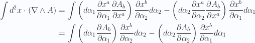
The differential form for our integral can now be computed by expanding out the dot product. We want

Evaluation of the interior dot products introduces the intrinsic antisymmetry required for Stokes theorem. For example, with

Since 
![\begin{aligned}( e_l \wedge e_k \wedge \cdots \wedge e_j \wedge e_i )\cdot(e^a \wedge e^b \wedge e^c \wedge \cdots e^d)={\delta^{[a}}_i{\delta^b}_j\cdots {\delta^{d]}}_l,\end{aligned} \hspace{\stretch{1}}(2.18)](https://s0.wp.com/latex.php?latex=%5Cbegin%7Baligned%7D%28+e_l+%5Cwedge+e_k+%5Cwedge+%5Ccdots+%5Cwedge+e_j+%5Cwedge+e_i+%29%5Ccdot%28e%5Ea+%5Cwedge+e%5Eb+%5Cwedge+e%5Ec+%5Cwedge+%5Ccdots+e%5Ed%29%3D%7B%5Cdelta%5E%7B%5Ba%7D%7D_i%7B%5Cdelta%5Eb%7D_j%5Ccdots+%7B%5Cdelta%5E%7Bd%5D%7D%7D_l%2C%5Cend%7Baligned%7D+%5Chspace%7B%5Cstretch%7B1%7D%7D%282.18%29&bg=fafcff&fg=2a2a2a&s=0&c=20201002)
and the curl integral takes it’s coordinate form
![\begin{aligned}\int d^n x \cdot ( \nabla \wedge A ) =\int d^n \alpha\frac{\partial {x^i}}{\partial {\alpha_1}}\frac{\partial {x^j}}{\partial {\alpha_2}}\cdots \frac{\partial {x^k}}{\partial {\alpha_{n-1}}}\frac{\partial {x^l}}{\partial {\alpha_n}}\partial_a A_{b c \cdots d}{\delta^{[a}}_i{\delta^b}_j\cdots {\delta^{d]}}_l.\end{aligned} \hspace{\stretch{1}}(2.19)](https://s0.wp.com/latex.php?latex=%5Cbegin%7Baligned%7D%5Cint+d%5En+x+%5Ccdot+%28+%5Cnabla+%5Cwedge+A+%29+%3D%5Cint+d%5En+%5Calpha%5Cfrac%7B%5Cpartial+%7Bx%5Ei%7D%7D%7B%5Cpartial+%7B%5Calpha_1%7D%7D%5Cfrac%7B%5Cpartial+%7Bx%5Ej%7D%7D%7B%5Cpartial+%7B%5Calpha_2%7D%7D%5Ccdots+%5Cfrac%7B%5Cpartial+%7Bx%5Ek%7D%7D%7B%5Cpartial+%7B%5Calpha_%7Bn-1%7D%7D%7D%5Cfrac%7B%5Cpartial+%7Bx%5El%7D%7D%7B%5Cpartial+%7B%5Calpha_n%7D%7D%5Cpartial_a+A_%7Bb+c+%5Ccdots+d%7D%7B%5Cdelta%5E%7B%5Ba%7D%7D_i%7B%5Cdelta%5Eb%7D_j%5Ccdots+%7B%5Cdelta%5E%7Bd%5D%7D%7D_l.%5Cend%7Baligned%7D+%5Chspace%7B%5Cstretch%7B1%7D%7D%282.19%29&bg=fafcff&fg=2a2a2a&s=0&c=20201002)
One final contraction of the paired indexes gives us our Stokes integral in its coordinate representation
![\begin{aligned}\boxed{\int d^n x \cdot ( \nabla \wedge A ) =\int d^n \alpha\frac{\partial {x^{[a}}}{\partial {\alpha_1}}\frac{\partial {x^b}}{\partial {\alpha_2}}\cdots \frac{\partial {x^c}}{\partial {\alpha_{n-1}}}\frac{\partial {x^{d]}}}{\partial {\alpha_n}}\partial_a A_{b c \cdots d}}\end{aligned} \hspace{\stretch{1}}(2.20)](https://s0.wp.com/latex.php?latex=%5Cbegin%7Baligned%7D%5Cboxed%7B%5Cint+d%5En+x+%5Ccdot+%28+%5Cnabla+%5Cwedge+A+%29+%3D%5Cint+d%5En+%5Calpha%5Cfrac%7B%5Cpartial+%7Bx%5E%7B%5Ba%7D%7D%7D%7B%5Cpartial+%7B%5Calpha_1%7D%7D%5Cfrac%7B%5Cpartial+%7Bx%5Eb%7D%7D%7B%5Cpartial+%7B%5Calpha_2%7D%7D%5Ccdots+%5Cfrac%7B%5Cpartial+%7Bx%5Ec%7D%7D%7B%5Cpartial+%7B%5Calpha_%7Bn-1%7D%7D%7D%5Cfrac%7B%5Cpartial+%7Bx%5E%7Bd%5D%7D%7D%7D%7B%5Cpartial+%7B%5Calpha_n%7D%7D%5Cpartial_a+A_%7Bb+c+%5Ccdots+d%7D%7D%5Cend%7Baligned%7D+%5Chspace%7B%5Cstretch%7B1%7D%7D%282.20%29&bg=fafcff&fg=2a2a2a&s=0&c=20201002)
We now have a starting point that is free of any of the abstraction of Geometric Algebra or differential forms. We can identify the products of partials here as components of a scalar hypervolume element (possibly signed depending on the orientation of the parametrization)
![\begin{aligned}d\alpha_1 d\alpha_2\cdots d\alpha_n\frac{\partial {x^{[a}}}{\partial {\alpha_1}}\frac{\partial {x^b}}{\partial {\alpha_2}}\cdots \frac{\partial {x^c}}{\partial {\alpha_{n-1}}}\frac{\partial {x^{d]}}}{\partial {\alpha_n}}\end{aligned} \hspace{\stretch{1}}(2.21)](https://s0.wp.com/latex.php?latex=%5Cbegin%7Baligned%7Dd%5Calpha_1+d%5Calpha_2%5Ccdots+d%5Calpha_n%5Cfrac%7B%5Cpartial+%7Bx%5E%7B%5Ba%7D%7D%7D%7B%5Cpartial+%7B%5Calpha_1%7D%7D%5Cfrac%7B%5Cpartial+%7Bx%5Eb%7D%7D%7B%5Cpartial+%7B%5Calpha_2%7D%7D%5Ccdots+%5Cfrac%7B%5Cpartial+%7Bx%5Ec%7D%7D%7B%5Cpartial+%7B%5Calpha_%7Bn-1%7D%7D%7D%5Cfrac%7B%5Cpartial+%7Bx%5E%7Bd%5D%7D%7D%7D%7B%5Cpartial+%7B%5Calpha_n%7D%7D%5Cend%7Baligned%7D+%5Chspace%7B%5Cstretch%7B1%7D%7D%282.21%29&bg=fafcff&fg=2a2a2a&s=0&c=20201002)
This is also a specific computation recipe for these hypervolume components, something that may not be obvious when we allow for general metrics for the space. We are also allowing for non-orthonormal coordinate representations, and arbitrary parametrization of the subspace that we are integrating over (our integral need not have the same dimension as the underlying vector space).
Observe that when the number of parameters equals the dimension of the space, we can write out the antisymmetric term utilizing the determinant of the Jacobian matrix
![\begin{aligned}\frac{\partial {x^{[a}}}{\partial {\alpha_1}}\frac{\partial {x^b}}{\partial {\alpha_2}}\cdots \frac{\partial {x^c}}{\partial {\alpha_{n-1}}}\frac{\partial {x^{d]}}}{\partial {\alpha_n}}= \epsilon^{a b \cdots d} {\left\lvert{ \frac{\partial(x^1, x^2, \cdots x^n)}{\partial(\alpha_1, \alpha_2, \cdots \alpha_n)} }\right\rvert}\end{aligned} \hspace{\stretch{1}}(2.22)](https://s0.wp.com/latex.php?latex=%5Cbegin%7Baligned%7D%5Cfrac%7B%5Cpartial+%7Bx%5E%7B%5Ba%7D%7D%7D%7B%5Cpartial+%7B%5Calpha_1%7D%7D%5Cfrac%7B%5Cpartial+%7Bx%5Eb%7D%7D%7B%5Cpartial+%7B%5Calpha_2%7D%7D%5Ccdots+%5Cfrac%7B%5Cpartial+%7Bx%5Ec%7D%7D%7B%5Cpartial+%7B%5Calpha_%7Bn-1%7D%7D%7D%5Cfrac%7B%5Cpartial+%7Bx%5E%7Bd%5D%7D%7D%7D%7B%5Cpartial+%7B%5Calpha_n%7D%7D%3D+%5Cepsilon%5E%7Ba+b+%5Ccdots+d%7D+%7B%5Cleft%5Clvert%7B+%5Cfrac%7B%5Cpartial%28x%5E1%2C+x%5E2%2C+%5Ccdots+x%5En%29%7D%7B%5Cpartial%28%5Calpha_1%2C+%5Calpha_2%2C+%5Ccdots+%5Calpha_n%29%7D+%7D%5Cright%5Crvert%7D%5Cend%7Baligned%7D+%5Chspace%7B%5Cstretch%7B1%7D%7D%282.22%29&bg=fafcff&fg=2a2a2a&s=0&c=20201002)
When the dimension of the space
![\begin{aligned}\frac{\partial {x^{[a_1}}}{\partial {\alpha_1}}\frac{\partial {x^{a_2}}}{\partial {\alpha_2}}\cdots \frac{\partial {x^{a_{n-1}}}}{\partial {\alpha_{n-1}}}\frac{\partial {x^{a_n]}}}{\partial {\alpha_n}}= {\left\lvert{ \frac{\partial(x^{a_1}, x^{a_2}, \cdots x^{a_n})}{\partial(\alpha_1, \alpha_2, \cdots \alpha_n)} }\right\rvert},\end{aligned} \hspace{\stretch{1}}(2.23)](https://s0.wp.com/latex.php?latex=%5Cbegin%7Baligned%7D%5Cfrac%7B%5Cpartial+%7Bx%5E%7B%5Ba_1%7D%7D%7D%7B%5Cpartial+%7B%5Calpha_1%7D%7D%5Cfrac%7B%5Cpartial+%7Bx%5E%7Ba_2%7D%7D%7D%7B%5Cpartial+%7B%5Calpha_2%7D%7D%5Ccdots+%5Cfrac%7B%5Cpartial+%7Bx%5E%7Ba_%7Bn-1%7D%7D%7D%7D%7B%5Cpartial+%7B%5Calpha_%7Bn-1%7D%7D%7D%5Cfrac%7B%5Cpartial+%7Bx%5E%7Ba_n%5D%7D%7D%7D%7B%5Cpartial+%7B%5Calpha_n%7D%7D%3D+%7B%5Cleft%5Clvert%7B+%5Cfrac%7B%5Cpartial%28x%5E%7Ba_1%7D%2C+x%5E%7Ba_2%7D%2C+%5Ccdots+x%5E%7Ba_n%7D%29%7D%7B%5Cpartial%28%5Calpha_1%2C+%5Calpha_2%2C+%5Ccdots+%5Calpha_n%29%7D+%7D%5Cright%5Crvert%7D%2C%5Cend%7Baligned%7D+%5Chspace%7B%5Cstretch%7B1%7D%7D%282.23%29&bg=fafcff&fg=2a2a2a&s=0&c=20201002)
however, we will have one such Jacobian for each unique choice of indexes.
The Stokes work starts here.
The task is to relate our integral to the boundary of this volume, coming up with an explicit recipe for the description of that bounding surface, and determining the exact form of the reduced rank integral. This job is essentially to reduce the ranks of the tensors that are being contracted in our Stokes integral. With the derivative applied to our rank
![\begin{aligned}\int d^n \alpha\frac{\partial {x^{[a}}}{\partial {\alpha_1}}\frac{\partial {x^b}}{\partial {\alpha_2}}\cdots \frac{\partial {x^c}}{\partial {\alpha_{n-1}}}\frac{\partial {x^{d]}}}{\partial {\alpha_n}}\partial_a A_{b c \cdots d} = ?\end{aligned} \hspace{\stretch{1}}(3.24)](https://s0.wp.com/latex.php?latex=%5Cbegin%7Baligned%7D%5Cint+d%5En+%5Calpha%5Cfrac%7B%5Cpartial+%7Bx%5E%7B%5Ba%7D%7D%7D%7B%5Cpartial+%7B%5Calpha_1%7D%7D%5Cfrac%7B%5Cpartial+%7Bx%5Eb%7D%7D%7B%5Cpartial+%7B%5Calpha_2%7D%7D%5Ccdots+%5Cfrac%7B%5Cpartial+%7Bx%5Ec%7D%7D%7B%5Cpartial+%7B%5Calpha_%7Bn-1%7D%7D%7D%5Cfrac%7B%5Cpartial+%7Bx%5E%7Bd%5D%7D%7D%7D%7B%5Cpartial+%7B%5Calpha_n%7D%7D%5Cpartial_a+A_%7Bb+c+%5Ccdots+d%7D+%3D+%3F%5Cend%7Baligned%7D+%5Chspace%7B%5Cstretch%7B1%7D%7D%283.24%29&bg=fafcff&fg=2a2a2a&s=0&c=20201002)
Now, while the setup here has been completely general, this task is motivated by study of special relativity, where there is a requirement to work in a four dimensional space. Because of that explicit goal, I’m not going to attempt to formulate this in a completely abstract fashion. That task is really one of introducing sufficiently general notation. Instead, I’m going to proceed with a simpleton approach, and do this explicitly, and repeatedly for each of the rank 1, rank 2, and rank 3 tensor cases. It will be clear how this all generalizes by doing so, should one wish to work in still higher dimensional spaces.
The rank 1 tensor case.
The equation we are working with for this vector case is
![\begin{aligned}\int d^2 x \cdot (\nabla \wedge A) =\int d{\alpha_1} d{\alpha_2}\frac{\partial {x^{[a}}}{\partial {\alpha_1}}\frac{\partial {x^{b]}}}{\partial {\alpha_2}}\partial_a A_{b}(\alpha_1, \alpha_2)\end{aligned} \hspace{\stretch{1}}(3.25)](https://s0.wp.com/latex.php?latex=%5Cbegin%7Baligned%7D%5Cint+d%5E2+x+%5Ccdot+%28%5Cnabla+%5Cwedge+A%29+%3D%5Cint+d%7B%5Calpha_1%7D+d%7B%5Calpha_2%7D%5Cfrac%7B%5Cpartial+%7Bx%5E%7B%5Ba%7D%7D%7D%7B%5Cpartial+%7B%5Calpha_1%7D%7D%5Cfrac%7B%5Cpartial+%7Bx%5E%7Bb%5D%7D%7D%7D%7B%5Cpartial+%7B%5Calpha_2%7D%7D%5Cpartial_a+A_%7Bb%7D%28%5Calpha_1%2C+%5Calpha_2%29%5Cend%7Baligned%7D+%5Chspace%7B%5Cstretch%7B1%7D%7D%283.25%29&bg=fafcff&fg=2a2a2a&s=0&c=20201002)
Expanding out the antisymmetric partials we have
![\begin{aligned}\frac{\partial {x^{[a}}}{\partial {\alpha_1}}\frac{\partial {x^{b]}}}{\partial {\alpha_2}} & =\frac{\partial {x^{a}}}{\partial {\alpha_1}}\frac{\partial {x^{b}}}{\partial {\alpha_2}}-\frac{\partial {x^{b}}}{\partial {\alpha_1}}\frac{\partial {x^{a}}}{\partial {\alpha_2}},\end{aligned}](https://s0.wp.com/latex.php?latex=%5Cbegin%7Baligned%7D%5Cfrac%7B%5Cpartial+%7Bx%5E%7B%5Ba%7D%7D%7D%7B%5Cpartial+%7B%5Calpha_1%7D%7D%5Cfrac%7B%5Cpartial+%7Bx%5E%7Bb%5D%7D%7D%7D%7B%5Cpartial+%7B%5Calpha_2%7D%7D+%26+%3D%5Cfrac%7B%5Cpartial+%7Bx%5E%7Ba%7D%7D%7D%7B%5Cpartial+%7B%5Calpha_1%7D%7D%5Cfrac%7B%5Cpartial+%7Bx%5E%7Bb%7D%7D%7D%7B%5Cpartial+%7B%5Calpha_2%7D%7D-%5Cfrac%7B%5Cpartial+%7Bx%5E%7Bb%7D%7D%7D%7B%5Cpartial+%7B%5Calpha_1%7D%7D%5Cfrac%7B%5Cpartial+%7Bx%5E%7Ba%7D%7D%7D%7B%5Cpartial+%7B%5Calpha_2%7D%7D%2C%5Cend%7Baligned%7D+&bg=fafcff&fg=2a2a2a&s=0&c=20201002)
with which we can reduce the integral to
Now, if it happens that

then each of the individual integrals in 

![\alpha_i \in [0,1]](https://s0.wp.com/latex.php?latex=%5Calpha_i+%5Cin+%5B0%2C1%5D&bg=fafcff&fg=2a2a2a&s=0&c=20201002)
![\begin{aligned}\begin{aligned} & \int d{\alpha_1} d{\alpha_2}\frac{\partial {x^{[a}}}{\partial {\alpha_1}}\frac{\partial {x^{b]}}}{\partial {\alpha_2}}\partial_a A_{b}(\alpha_1, \alpha_2) \\ & =\int \left( A_b(1, \alpha_2) - A_b(0, \alpha_2) \right)\frac{\partial {x^{b}}}{\partial {\alpha_2}} d{\alpha_2}-\left( A_b(\alpha_1, 1) - A_b(\alpha_1, 0) \right)\frac{\partial {x^{b}}}{\partial {\alpha_1}} d{\alpha_1}.\end{aligned}\end{aligned} \hspace{\stretch{1}}(3.27)](https://s0.wp.com/latex.php?latex=%5Cbegin%7Baligned%7D%5Cbegin%7Baligned%7D+%26+%5Cint+d%7B%5Calpha_1%7D+d%7B%5Calpha_2%7D%5Cfrac%7B%5Cpartial+%7Bx%5E%7B%5Ba%7D%7D%7D%7B%5Cpartial+%7B%5Calpha_1%7D%7D%5Cfrac%7B%5Cpartial+%7Bx%5E%7Bb%5D%7D%7D%7D%7B%5Cpartial+%7B%5Calpha_2%7D%7D%5Cpartial_a+A_%7Bb%7D%28%5Calpha_1%2C+%5Calpha_2%29+%5C%5C+%26+%3D%5Cint+%5Cleft%28+A_b%281%2C+%5Calpha_2%29+-+A_b%280%2C+%5Calpha_2%29+%5Cright%29%5Cfrac%7B%5Cpartial+%7Bx%5E%7Bb%7D%7D%7D%7B%5Cpartial+%7B%5Calpha_2%7D%7D+d%7B%5Calpha_2%7D-%5Cleft%28+A_b%28%5Calpha_1%2C+1%29+-+A_b%28%5Calpha_1%2C+0%29+%5Cright%29%5Cfrac%7B%5Cpartial+%7Bx%5E%7Bb%7D%7D%7D%7B%5Cpartial+%7B%5Calpha_1%7D%7D+d%7B%5Calpha_1%7D.%5Cend%7Baligned%7D%5Cend%7Baligned%7D+%5Chspace%7B%5Cstretch%7B1%7D%7D%283.27%29&bg=fafcff&fg=2a2a2a&s=0&c=20201002)
It’s also fairly common to see 
![\begin{aligned}\int d{\alpha_1} d{\alpha_2}\frac{\partial {x^{[a}}}{\partial {\alpha_1}}\frac{\partial {x^{b]}}}{\partial {\alpha_2}}\partial_a A_{b}(\alpha_1, \alpha_2)=\int {\left.{{A_b}}\right\vert}_{{\partial \alpha_1}}\frac{\partial {x^{b}}}{\partial {\alpha_2}} d{\alpha_2}-{\left.{{A_b}}\right\vert}_{{\partial \alpha_2}}\frac{\partial {x^{b}}}{\partial {\alpha_1}} d{\alpha_1}.\end{aligned} \hspace{\stretch{1}}(3.28)](https://s0.wp.com/latex.php?latex=%5Cbegin%7Baligned%7D%5Cint+d%7B%5Calpha_1%7D+d%7B%5Calpha_2%7D%5Cfrac%7B%5Cpartial+%7Bx%5E%7B%5Ba%7D%7D%7D%7B%5Cpartial+%7B%5Calpha_1%7D%7D%5Cfrac%7B%5Cpartial+%7Bx%5E%7Bb%5D%7D%7D%7D%7B%5Cpartial+%7B%5Calpha_2%7D%7D%5Cpartial_a+A_%7Bb%7D%28%5Calpha_1%2C+%5Calpha_2%29%3D%5Cint+%7B%5Cleft.%7B%7BA_b%7D%7D%5Cright%5Cvert%7D_%7B%7B%5Cpartial+%5Calpha_1%7D%7D%5Cfrac%7B%5Cpartial+%7Bx%5E%7Bb%7D%7D%7D%7B%5Cpartial+%7B%5Calpha_2%7D%7D+d%7B%5Calpha_2%7D-%7B%5Cleft.%7B%7BA_b%7D%7D%5Cright%5Cvert%7D_%7B%7B%5Cpartial+%5Calpha_2%7D%7D%5Cfrac%7B%5Cpartial+%7Bx%5E%7Bb%7D%7D%7D%7B%5Cpartial+%7B%5Calpha_1%7D%7D+d%7B%5Calpha_1%7D.%5Cend%7Baligned%7D+%5Chspace%7B%5Cstretch%7B1%7D%7D%283.28%29&bg=fafcff&fg=2a2a2a&s=0&c=20201002)
Also note that since we are summing over all 
![\begin{aligned}\frac{\partial {x^{[a}}}{\partial {\alpha_1}}\frac{\partial {x^{b]}}}{\partial {\alpha_2}}=-\frac{\partial {x^{[b}}}{\partial {\alpha_1}}\frac{\partial {x^{a]}}}{\partial {\alpha_2}},\end{aligned} \hspace{\stretch{1}}(3.29)](https://s0.wp.com/latex.php?latex=%5Cbegin%7Baligned%7D%5Cfrac%7B%5Cpartial+%7Bx%5E%7B%5Ba%7D%7D%7D%7B%5Cpartial+%7B%5Calpha_1%7D%7D%5Cfrac%7B%5Cpartial+%7Bx%5E%7Bb%5D%7D%7D%7D%7B%5Cpartial+%7B%5Calpha_2%7D%7D%3D-%5Cfrac%7B%5Cpartial+%7Bx%5E%7B%5Bb%7D%7D%7D%7B%5Cpartial+%7B%5Calpha_1%7D%7D%5Cfrac%7B%5Cpartial+%7Bx%5E%7Ba%5D%7D%7D%7D%7B%5Cpartial+%7B%5Calpha_2%7D%7D%2C%5Cend%7Baligned%7D+%5Chspace%7B%5Cstretch%7B1%7D%7D%283.29%29&bg=fafcff&fg=2a2a2a&s=0&c=20201002)
we can write this summing over all unique pairs of
![\begin{aligned}\boxed{\sum_{a < b}\int d{\alpha_1} d{\alpha_2}\frac{\partial {x^{[a}}}{\partial {\alpha_1}}\frac{\partial {x^{b]}}}{\partial {\alpha_2}}\left( \partial_a A_{b}-\partial_b A_{a} \right)=\int {\left.{{A_b}}\right\vert}_{{\partial \alpha_1}}\frac{\partial {x^{b}}}{\partial {\alpha_2}} d{\alpha_2}-{\left.{{A_b}}\right\vert}_{{\partial \alpha_2}}\frac{\partial {x^{b}}}{\partial {\alpha_1}} d{\alpha_1}.}\end{aligned} \hspace{\stretch{1}}(3.30)](https://s0.wp.com/latex.php?latex=%5Cbegin%7Baligned%7D%5Cboxed%7B%5Csum_%7Ba+%3C+b%7D%5Cint+d%7B%5Calpha_1%7D+d%7B%5Calpha_2%7D%5Cfrac%7B%5Cpartial+%7Bx%5E%7B%5Ba%7D%7D%7D%7B%5Cpartial+%7B%5Calpha_1%7D%7D%5Cfrac%7B%5Cpartial+%7Bx%5E%7Bb%5D%7D%7D%7D%7B%5Cpartial+%7B%5Calpha_2%7D%7D%5Cleft%28+%5Cpartial_a+A_%7Bb%7D-%5Cpartial_b+A_%7Ba%7D+%5Cright%29%3D%5Cint+%7B%5Cleft.%7B%7BA_b%7D%7D%5Cright%5Cvert%7D_%7B%7B%5Cpartial+%5Calpha_1%7D%7D%5Cfrac%7B%5Cpartial+%7Bx%5E%7Bb%7D%7D%7D%7B%5Cpartial+%7B%5Calpha_2%7D%7D+d%7B%5Calpha_2%7D-%7B%5Cleft.%7B%7BA_b%7D%7D%5Cright%5Cvert%7D_%7B%7B%5Cpartial+%5Calpha_2%7D%7D%5Cfrac%7B%5Cpartial+%7Bx%5E%7Bb%7D%7D%7D%7B%5Cpartial+%7B%5Calpha_1%7D%7D+d%7B%5Calpha_1%7D.%7D%5Cend%7Baligned%7D+%5Chspace%7B%5Cstretch%7B1%7D%7D%283.30%29&bg=fafcff&fg=2a2a2a&s=0&c=20201002)
In this form we have recovered the original geometric structure, with components of the curl multiplied by the component of the area element that shares the orientation and direction of that portion of the curl bivector.
This form of the result with evaluation at the boundaries in this form, assumed that 


![\begin{aligned}\boxed{\sum_{a < b}\int d{\alpha_1} d{\alpha_2}\frac{\partial {x^{[a}}}{\partial {\alpha_1}}\frac{\partial {x^{b]}}}{\partial {\alpha_2}}\left( \partial_a A_{b}-\partial_b A_{a} \right)=\int d\alpha_2\int d\alpha_1\frac{\partial {A_b}}{\partial {\alpha_1}}\frac{\partial {x^{b}}}{\partial {\alpha_2}}-\int d\alpha_2\int d\alpha_1\frac{\partial {A_b}}{\partial {\alpha_2}}\frac{\partial {x^{b}}}{\partial {\alpha_1}}}\end{aligned} \hspace{\stretch{1}}(3.31)](https://s0.wp.com/latex.php?latex=%5Cbegin%7Baligned%7D%5Cboxed%7B%5Csum_%7Ba+%3C+b%7D%5Cint+d%7B%5Calpha_1%7D+d%7B%5Calpha_2%7D%5Cfrac%7B%5Cpartial+%7Bx%5E%7B%5Ba%7D%7D%7D%7B%5Cpartial+%7B%5Calpha_1%7D%7D%5Cfrac%7B%5Cpartial+%7Bx%5E%7Bb%5D%7D%7D%7D%7B%5Cpartial+%7B%5Calpha_2%7D%7D%5Cleft%28+%5Cpartial_a+A_%7Bb%7D-%5Cpartial_b+A_%7Ba%7D+%5Cright%29%3D%5Cint+d%5Calpha_2%5Cint+d%5Calpha_1%5Cfrac%7B%5Cpartial+%7BA_b%7D%7D%7B%5Cpartial+%7B%5Calpha_1%7D%7D%5Cfrac%7B%5Cpartial+%7Bx%5E%7Bb%7D%7D%7D%7B%5Cpartial+%7B%5Calpha_2%7D%7D-%5Cint+d%5Calpha_2%5Cint+d%5Calpha_1%5Cfrac%7B%5Cpartial+%7BA_b%7D%7D%7B%5Cpartial+%7B%5Calpha_2%7D%7D%5Cfrac%7B%5Cpartial+%7Bx%5E%7Bb%7D%7D%7D%7B%5Cpartial+%7B%5Calpha_1%7D%7D%7D%5Cend%7Baligned%7D+%5Chspace%7B%5Cstretch%7B1%7D%7D%283.31%29&bg=fafcff&fg=2a2a2a&s=0&c=20201002)
Can this be reduced any further in the general case? Having seen the statements of Stokes theorem in it’s differential forms formulation, I initially expected the answer was yes, and only when I got to evaluating my 
Sanity check:  case in rectangular coordinates.
For 
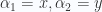

Our RHS expands to

We have

The RHS is just a positively oriented line integral around the rectangle of integration

This special case is also recognizable as Green’s theorem, evident with the substitution 


Strictly speaking, Green’s theorem is more general, since it applies to integration regions more general than rectangles, but that generalization can be arrived at easily enough, once the region is broken down into adjoining elementary regions.
Sanity check:  case in rectangular coordinates.
It is expected that we can recover the classical Kelvin-Stokes theorem if we use rectangular coordinates in 
Note that we cannot just add these to form a complete integral 
All that said, we shouldn’t actually have to go to all this work. Instead we can stick to a two variable parametrization of the surface, and use 3.30 directly.
An illustration for a spacetime surface.
Suppose we have a particle trajectory defined by an active Lorentz transformation from an initial spacetime point

Let the Lorentz transformation be formed by a composition of boost and rotation

Different rates of evolution of 


We can compute displacements along the trajectories formed by keeping either
Writing 
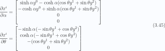
Different choices of the initial point 

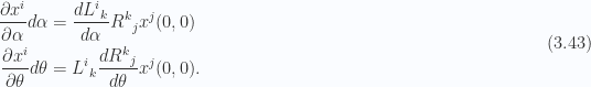
We can now compute our Jacobian determinants
![\begin{aligned}\frac{\partial {x^{[a}}}{\partial {\alpha}} \frac{\partial {x^{b]}}}{\partial {\theta}}={\left\lvert{\frac{\partial(x^a, x^b)}{\partial(\alpha, \theta)}}\right\rvert}.\end{aligned} \hspace{\stretch{1}}(3.49)](https://s0.wp.com/latex.php?latex=%5Cbegin%7Baligned%7D%5Cfrac%7B%5Cpartial+%7Bx%5E%7B%5Ba%7D%7D%7D%7B%5Cpartial+%7B%5Calpha%7D%7D+%5Cfrac%7B%5Cpartial+%7Bx%5E%7Bb%5D%7D%7D%7D%7B%5Cpartial+%7B%5Ctheta%7D%7D%3D%7B%5Cleft%5Clvert%7B%5Cfrac%7B%5Cpartial%28x%5Ea%2C+x%5Eb%29%7D%7B%5Cpartial%28%5Calpha%2C+%5Ctheta%29%7D%7D%5Cright%5Crvert%7D.%5Cend%7Baligned%7D+%5Chspace%7B%5Cstretch%7B1%7D%7D%283.49%29&bg=fafcff&fg=2a2a2a&s=0&c=20201002)
Those are

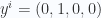
Using this, let’s see a specific 4D example in spacetime for the integral of the curl of some four vector 

The LHS is thus found to be
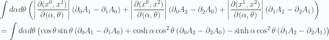
On the RHS we have

Because of the complexity of the surface, only the second term on the RHS has the “evaluate on the boundary” characteristic that may have been expected from a Green’s theorem like line integral.
It is also worthwhile to point out that we have had to be very careful with upper and lower indexes all along (and have done so with the expectation that our application would include the special relativity case where our metric determinant is minus one.) Because we worked with upper indexes for the area element, we had to work with lower indexes for the four vector and the components of the gradient that we included in our curl evaluation.
The rank 2 tensor case.
Let’s consider briefly the terms in the contraction sum

For any choice of a set of three distinct indexes 


Observe that we have no sign alternation like we had in the vector (rank 1 tensor) case. That sign alternation in this summation expansion appears to occur only for odd grade tensors.
Returning to the problem, we wish to expand the determinant in order to apply a chain rule contraction as done in the rank-1 case. This can be done along any of rows or columns of the determinant, and we can write any of
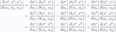
This allows the contraction of the index 
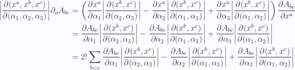
Dividing out the common 
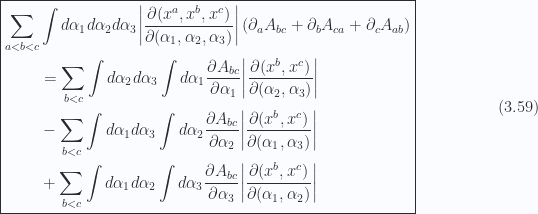
In general, as observed in the spacetime surface example above, the two index Jacobians can be functions of the integration variable first being eliminated. In the special cases where this is not the case (such as the 
The rank 3 tensor case.
The key step is once again just a determinant expansion

so that the sum can be reduced from a four index contraction to a 3 index contraction

That’s the essence of the theorem, but we can play the same combinatorial reduction games to reduce the built in redundancy in the result

A note on Four diverence.
Our four divergence integral has the following form

We can relate this to the rank 3 Stokes theorem with a duality transformation, multiplying with a pseudoscalar

where 

The divergence integral in terms of the rank 3 tensor is

and we are free to perform the same Stokes reduction of the integral. Of course, this is particularly simple in rectangular coordinates. I still have to think though one sublty that I feel may be important. We could have started off with an integral of the following form

and I think this differs from our starting point slightly because this has none of the antisymmetric structure of the signed 4 volume element that we have used. We do not take the absolute value of our Jacobians anywhere.
